This QuickStart presents common challenges when working with dates. Sigma can be used to manipulate dates to get the desired results, quickly and easily.
There are many ways to work with dates in Sigma. Not every solution is covered and you may even find a better method. Suggestions and feedback are always appreciated.
This QuickStart assumes you have a working instance of Sigma and the connection called Sigma Sample Database.
We will use the Sigma-provided RETAIL.PLUGS_ELECTRONICS.PLUGS_ELECTRONICS_HANDS_ON_LAB_DATA table so you can follow along and recreate each step in your own Sigma environment.
Target Audience
Sigma builders looking for solutions to date challenges or who just wants to learn new date methods.
Prerequisites
- Any modern browser is acceptable.
- Access to your Sigma environment.
- Some familiarity with Sigma is assumed. Not all steps are shown, as basic Sigma functionality is assumed.

Let's start with the standard ways to adjust a date column.
Log into Sigma, click Create new and select Workbook.
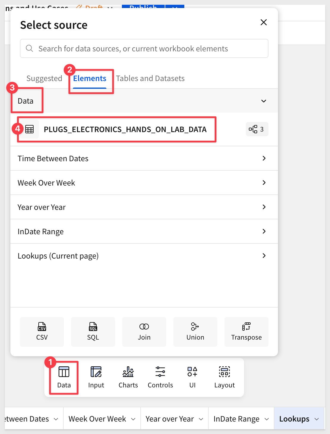
From the Element bar, under the Data group, place a new Table on the page.
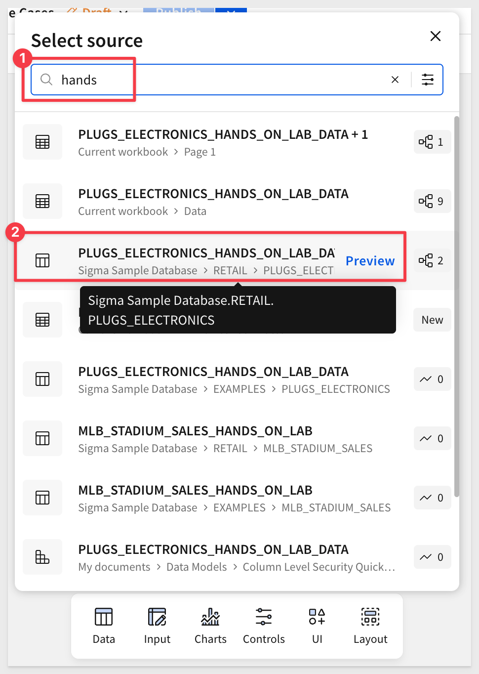
Click Select source for the new table.
Search for Hands and select the PLUGS_ELECTRONICS_HANDS_ON_LAB_DATA table from the RETAIL database.
Save the workbook as Common Date Functions and Use Cases.
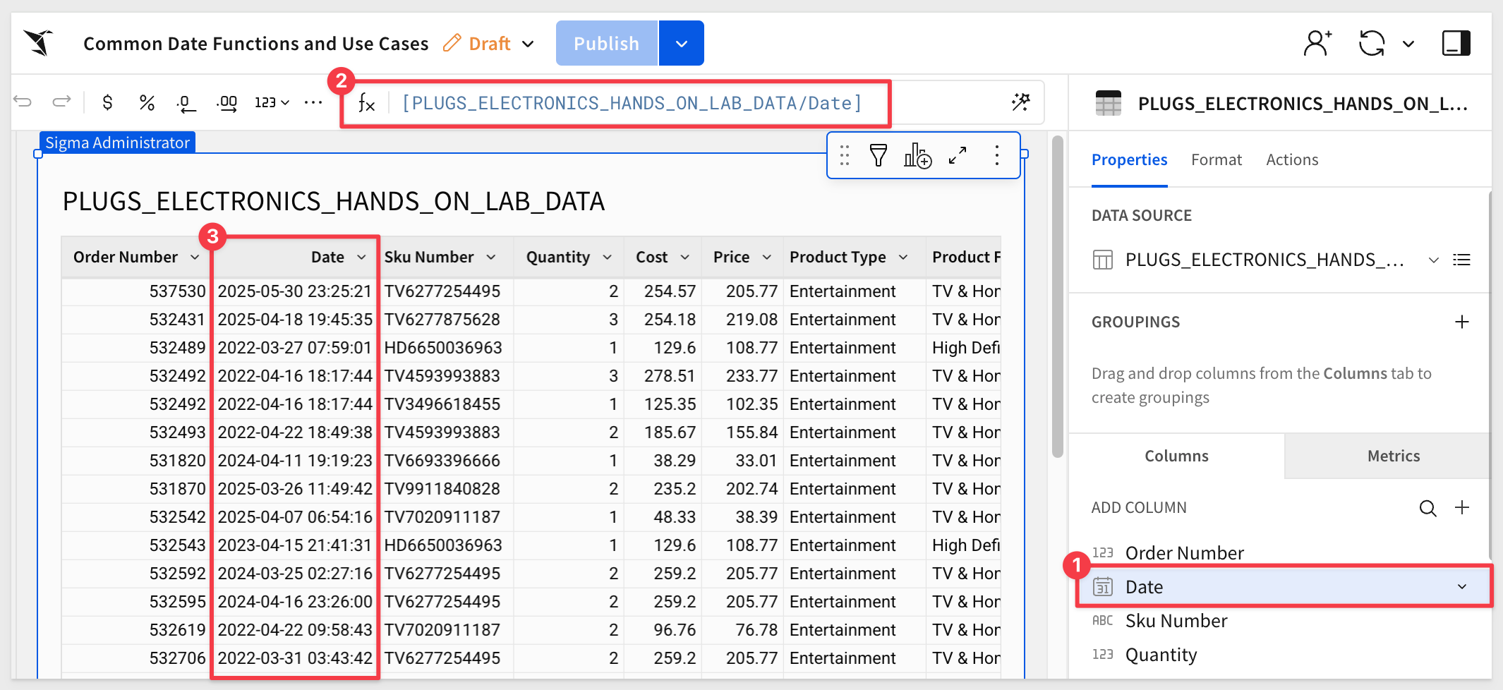
We're primarily interested in the Date column, which is coming in ‘as-is' from the warehouse:
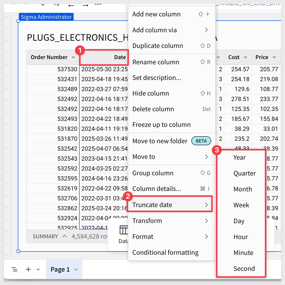
Click on the Date column down arrow and select Truncate date. This is one way to modify how the Date column is displayed.
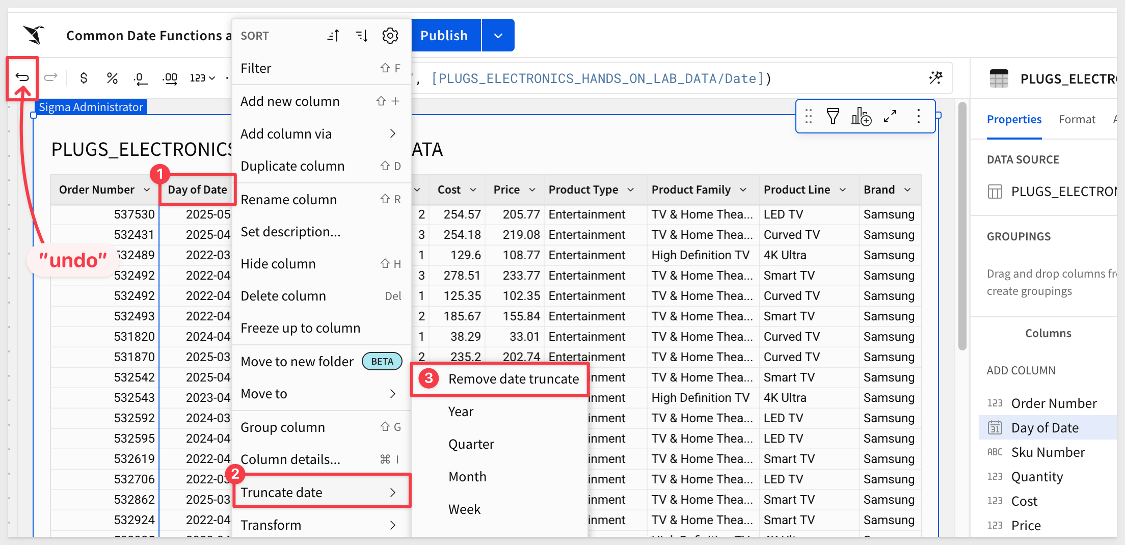
If you select the Day option, you'll see the column name changes to Day of Date.
Reset the Date column back to the default. You can use Remove date truncate from the column's menu but the Undo icon is faster:
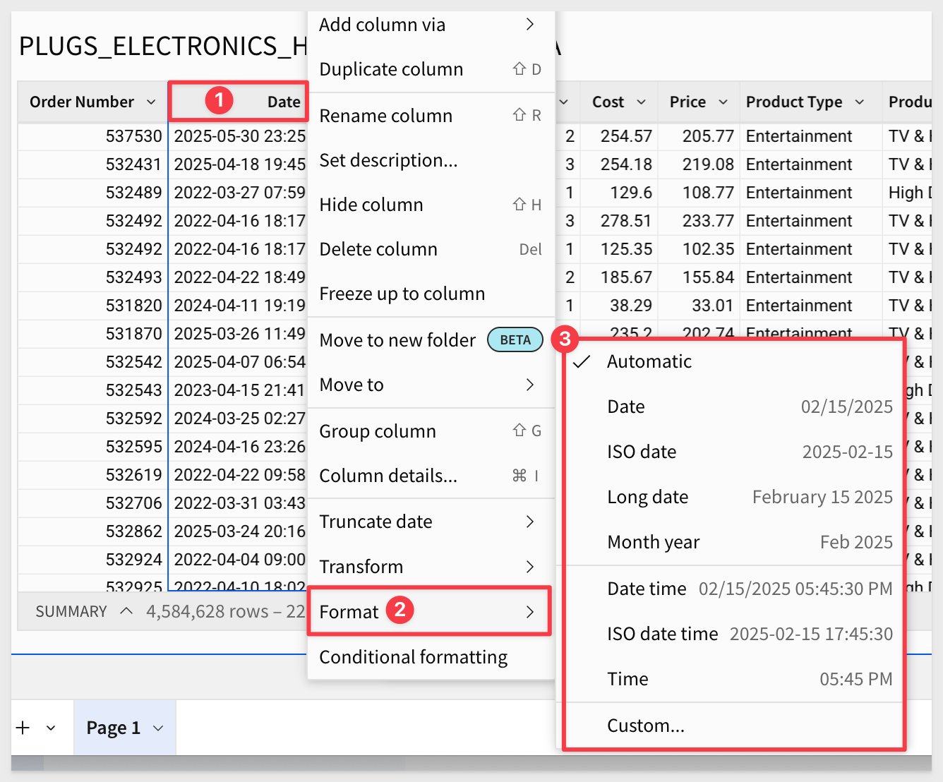
Click on the Date column down arrow and select Format date. This is another way to change how the Date column is displayed:
Feel free to experiment with the available options, resetting to the original when done.
Sigma supports applying custom formats to date columns. You can do this by selecting the Date column menu and then Format > Custom:
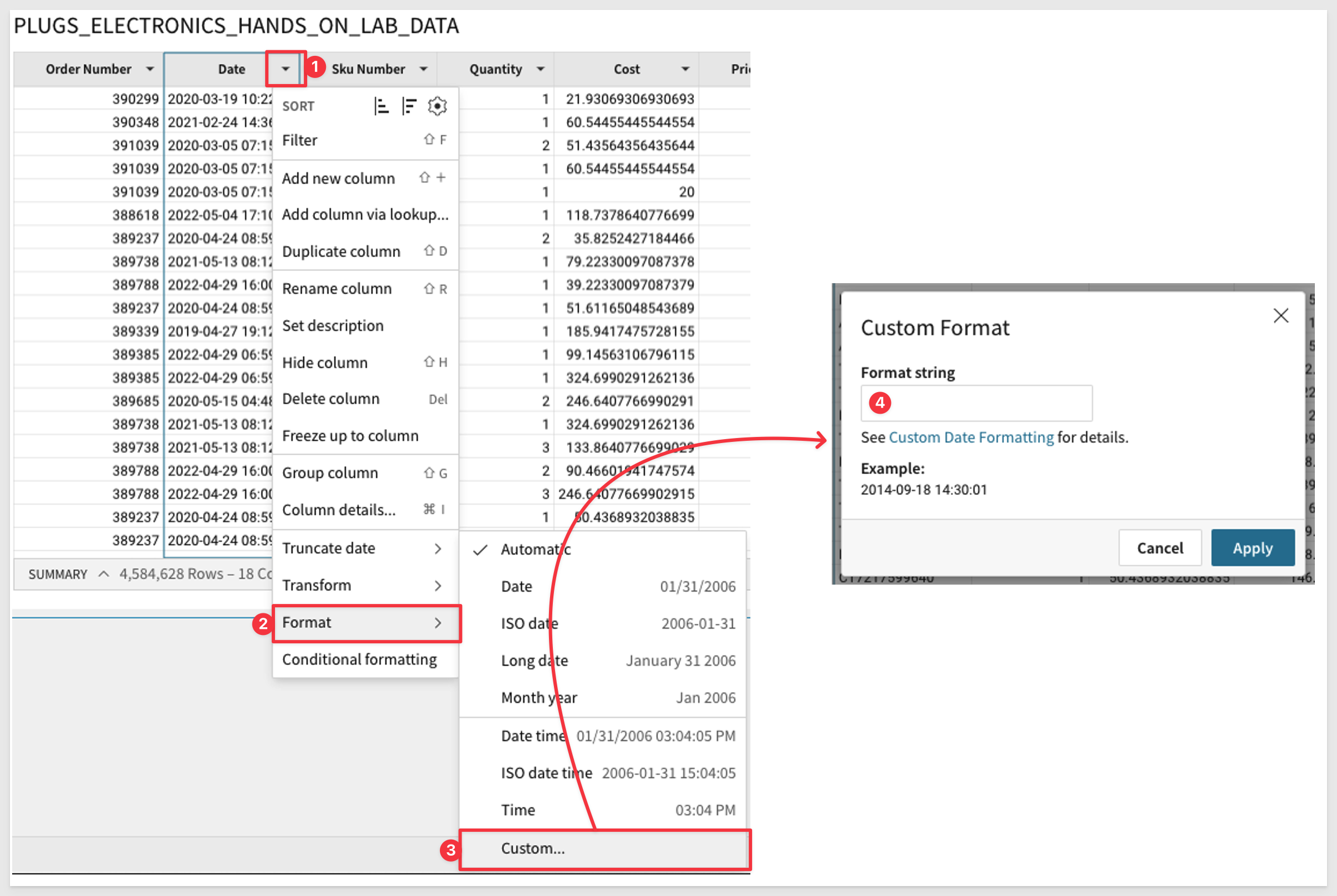
Entering the format string below will show a sample output in the popup:
%a %B %d %Y
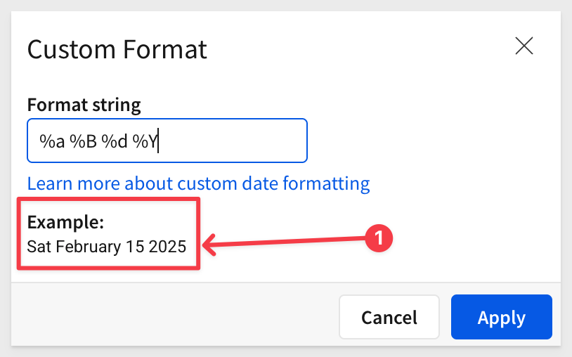
This helps confirm your format string is correct before applying it.
Feel free to experiment, then reset the Date column back to the default when done.
The formula bar
Another way to apply custom date formatting is by using the formula bar and the DateFormat function.
For example, you may want to get the full month name from a date column.
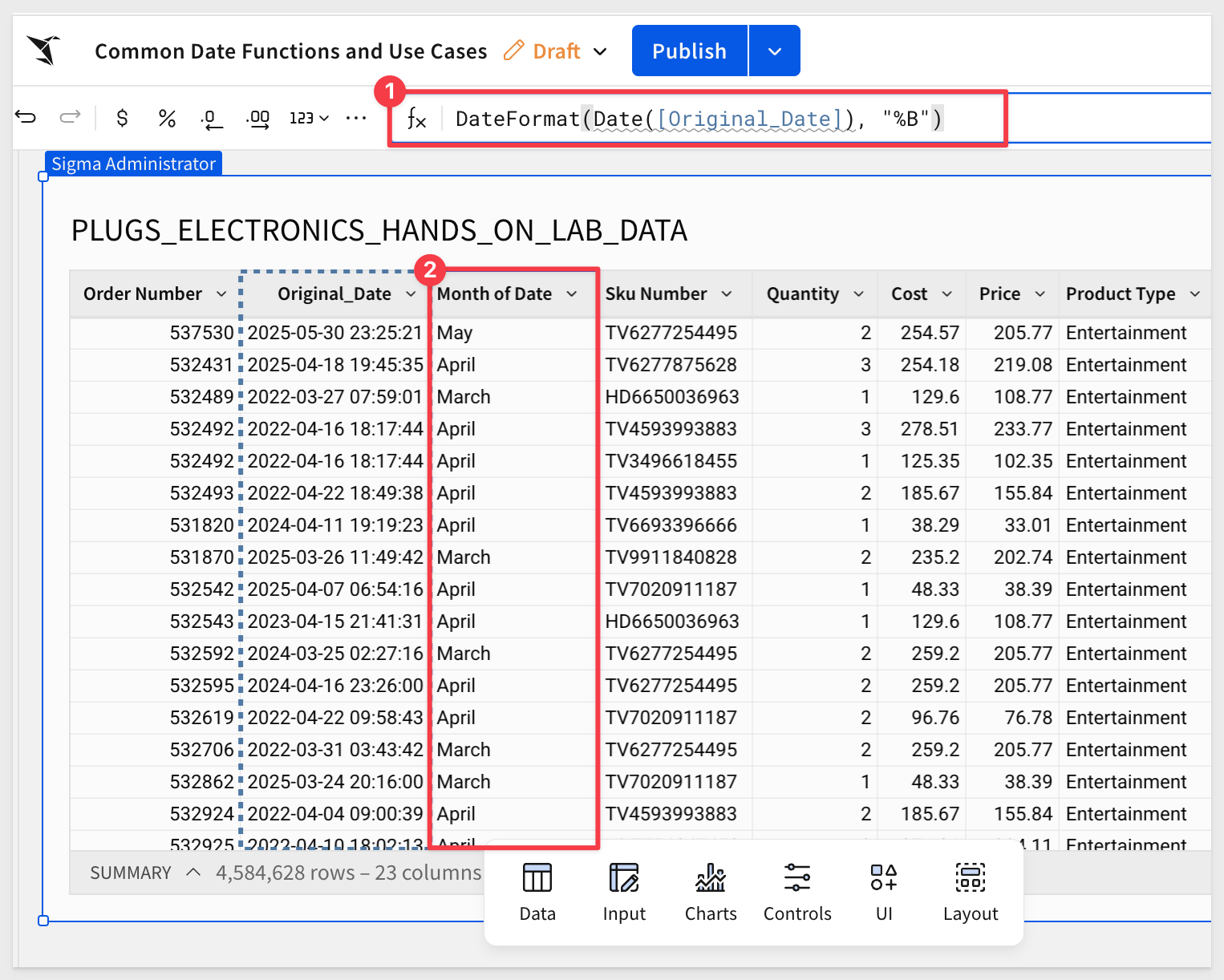
Create a new column by using the Date columns menu and selecting Add new column. Rename the new column Month of Date.
To make it clear for users, rename the Date column to Original_Date.
Click the Month of Date column, enter this formula into the formula bar and press enter.
DateFormat(Date([Original_Date]), "%B")
This demonstrates how to use the formula bar to apply both a function (DateFormat) and a custom format string:
Here are a few other examples created using the same method—many more are possible:
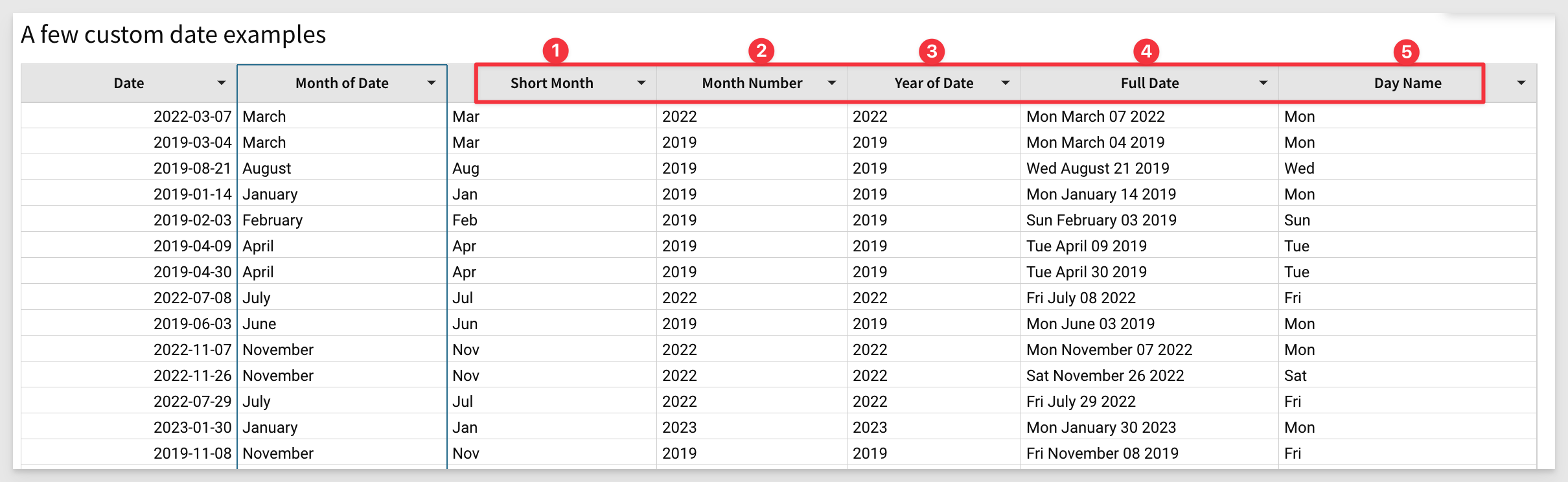
For more information, see Custom format strings
Now that we've covered the basics, let's apply what we've learned to a new use case.
For example, it's often useful for users to know the Effective Business Day an order was placed. If an order is placed on a Saturday or Sunday, this column will show Friday as the effective day, helping analysts align reporting with standard business operations.
Undo any changes we made to our table, and then format the Date column to basic Date format:
Rename the Date column to Today to make its purpose clearer to users.
Next, we want to display the weekday name for each value in the Today column.
Add a new column next to Today, and set its formula to:
DateFormat(Date([Today]), "%A")
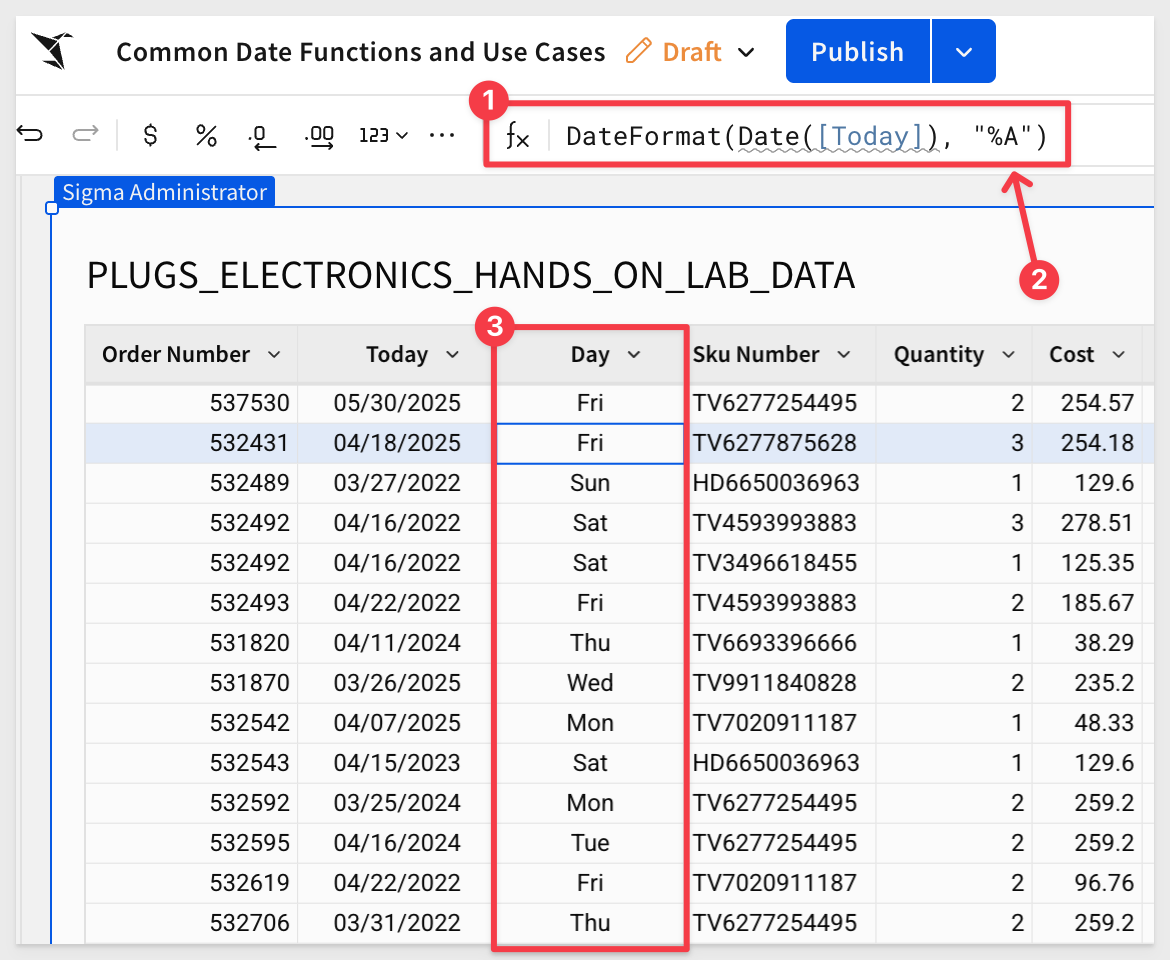
Now that we have the current weekday name, we can apply it to the use case.
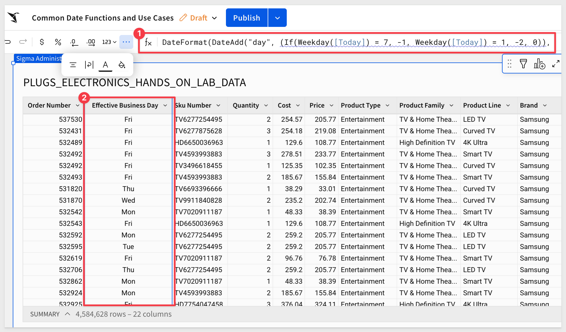
Add another new column next to Day and use the following formula:
DateFormat(DateAdd("day", (If(Weekday([Today]) = 7, -1, Weekday([Today]) = 1, -2, 0)), [Today]), "%A")
This formula returns the previous weekday name if today is Saturday (7) or Sunday (1); otherwise, it returns today's name.
Then, hide the Today and Day columns, and rename the new column to Effective Business Day:
For more information, see Define custom datetime formats
Click Publish.
s often useful to measure the time elapsed between two dates (or timestamps). Some examples are:
Call Center Support: Call duration
Customer Service: Order fulfillment time
Healthcare: Time since last blood test
Let's take a look at the customer service use case.
Marketing is interested in targeting customers who purchase frequently but only has a table with all orders to start with.
They want to answer a few key questions:
- When was a customer's first order?
- When was their second order?
- Number of days between the first and second order?
- How long since they last placed an order?
- Marketing will use this in campaigns targeting active and inactive customers.
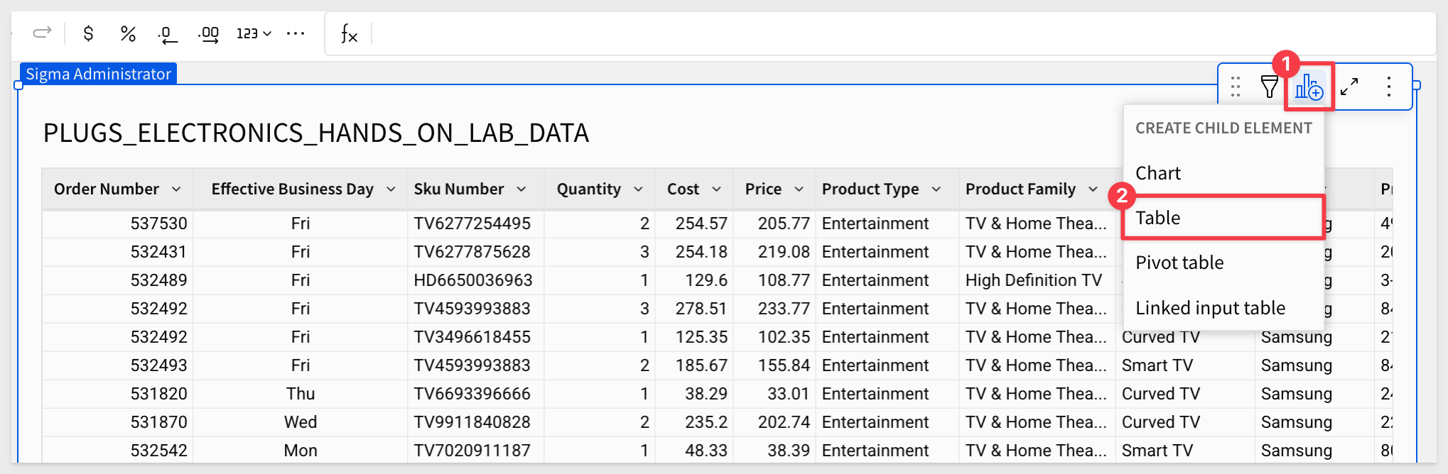
We'll continue using the PLUGS_ELECTRONICS_HANDS_ON_LAB_DATA table, but this time we'll create a child table.
Rename the child table Time Between Dates and move it to a new workbook page:
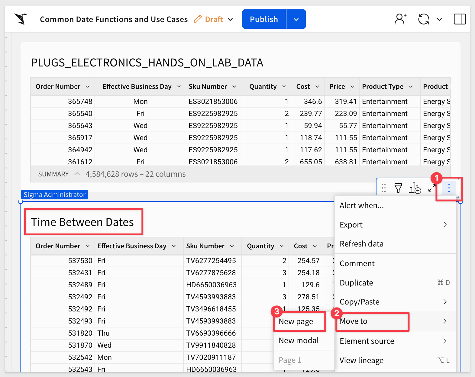
Rename the new workbook page Time Between Dates.
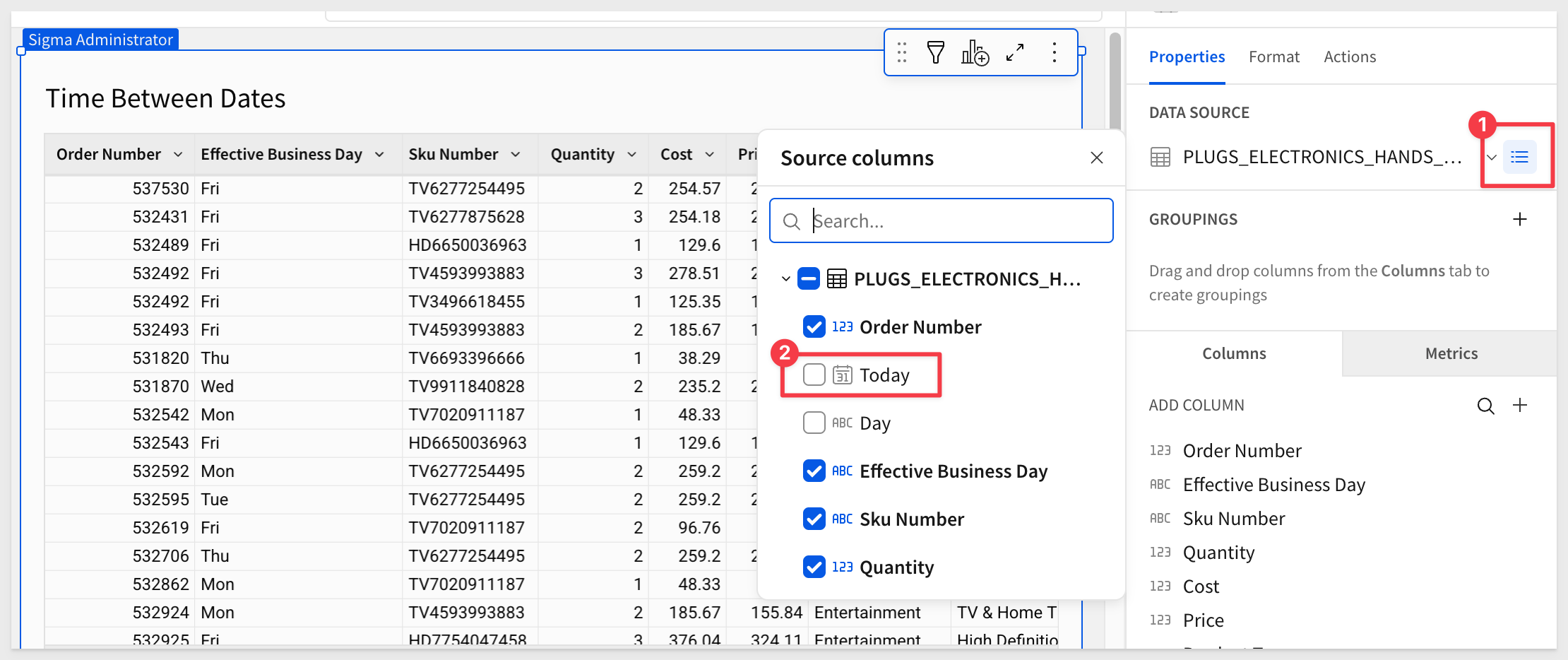
We only need a few columns including the Today column but that is hidden from our last section. No problem—it's still available in the child table, and we can make it visible:
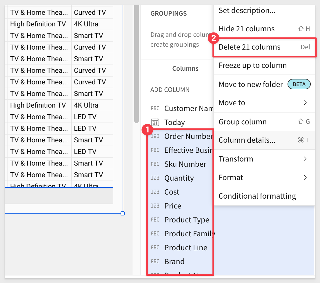
Since we don't need most columns in the child table, we can delete them, leaving only the Customer Name and Today columns.
Using the Element panel, move the Customer Name and Today columns to the top of the list and then select all others and click Delete 21 columns:
Drag the Customer Name column to GROUP BY.
Drag the Customer Name column to GROUPINGS to create a new group.
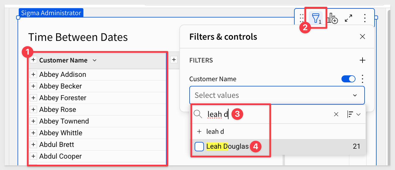
To simplify the view, filter the data where Customer Name = Leah Douglas:
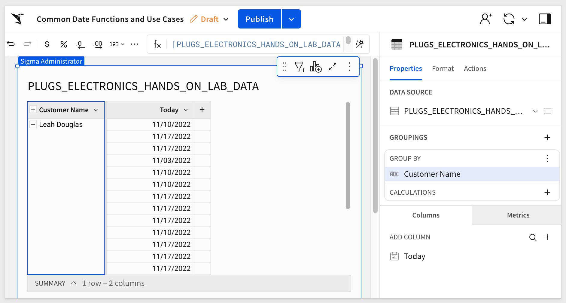
The table should now look like this:
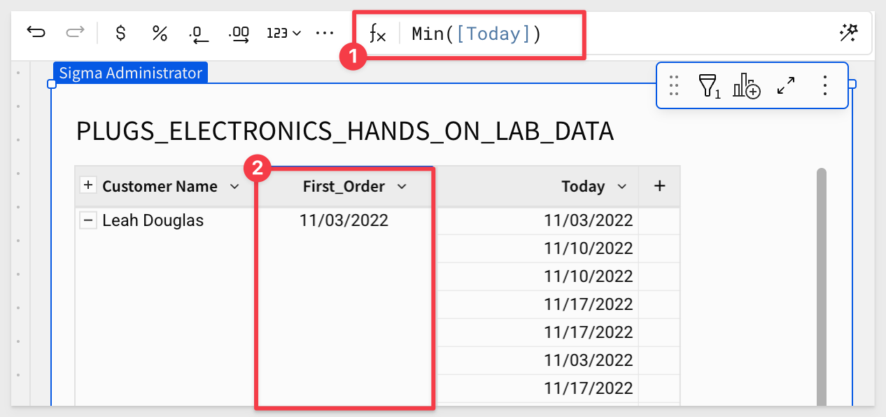
Add a new column next to Customer Name and rename it to First_Order.
For First_Order set the formula to:
Min([Today])
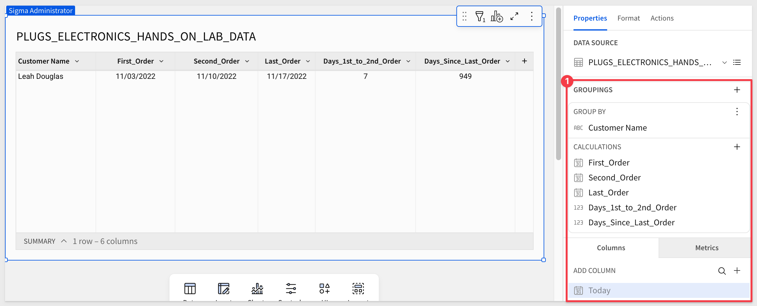
Now add four more columns, renaming them and applying the following formulas:
For more information, see Keyboard shortcuts: Microsoft Windows or Keyboard shortcuts: Mac OS
Column Name:                    Formula:
Second_Order                    Nth([Today], 2)
Last_Order                      Max([Today])
Days_1st_to_2nd_Order           DateDiff("day", [First_Order], [Second_Order])
Days_Since_Last_Order           DateDiff("day", [Last_Order], Today())
Hide the Today column.
The table should now look like this:
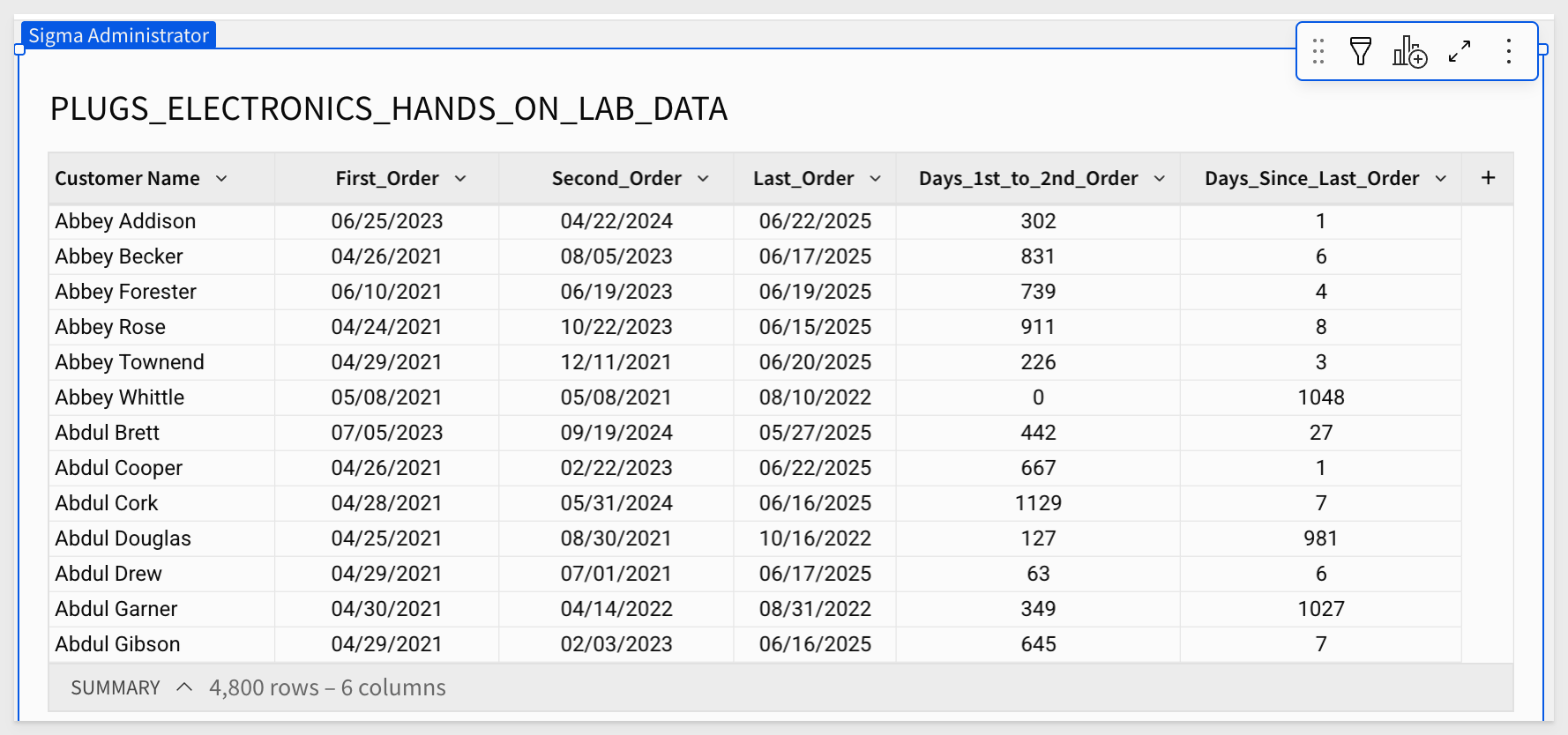
Go ahead and disable the filter.
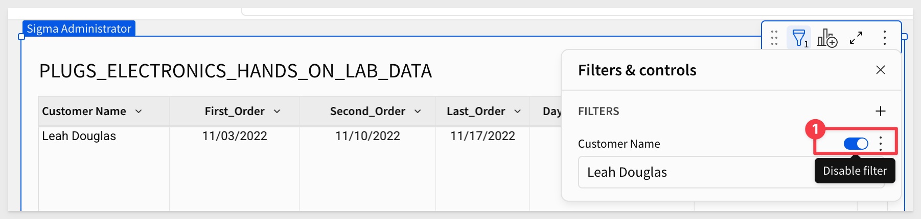
Marketing now has the data they requested:
Sales Operations wants to see how weekly sales numbers look compared to the previous week.
Let's use this example to explore Sigma's Lead and Lag functions. These functions make this type of comparison surprisingly easy.
In this example, we'll approach the data a bit differently this time. Create another Workbook Page and rename it Week Over Week.
Add a table to the page, and this time select F_Sales from the Sigma Sample Database.
This gives us all the sales transactions.
Next, we'll join another table to bring in point-of-sale data.
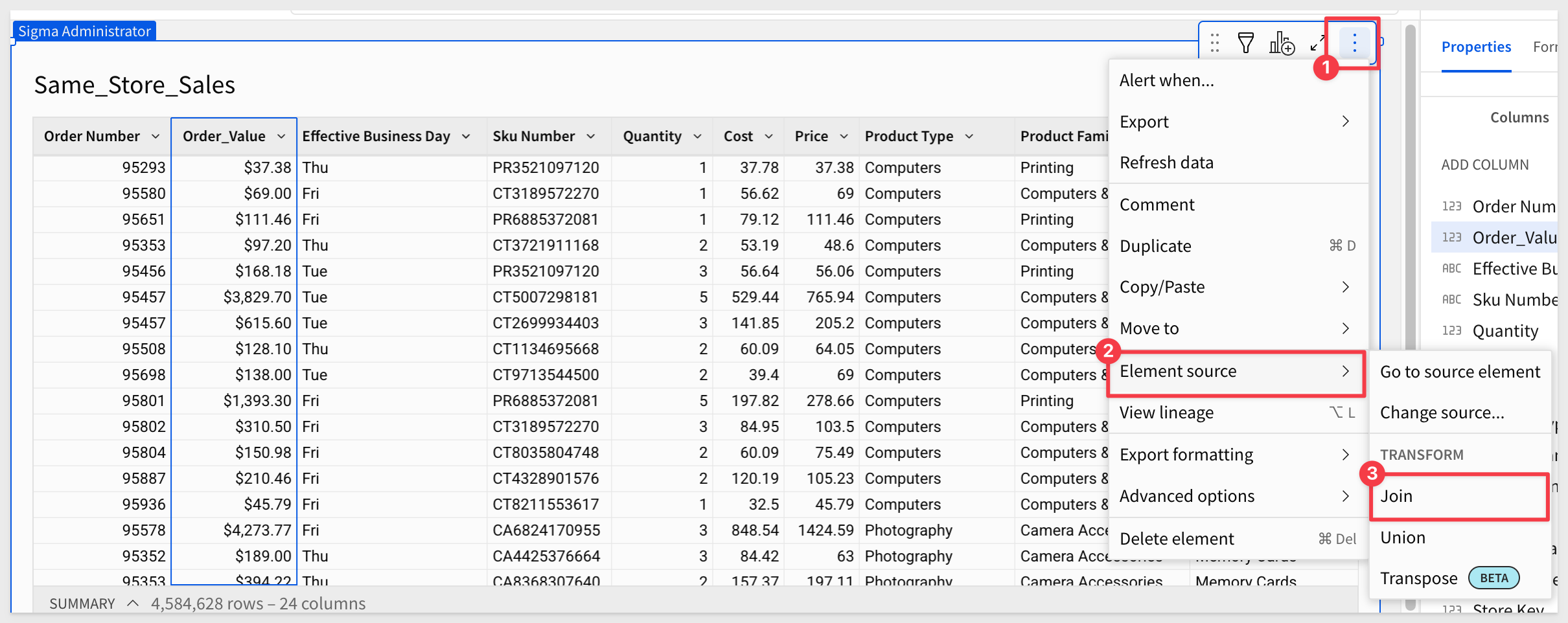
Click the 3-dot menu on the F_Sales table and select Element Source and then Join:

Search for and select F_Point_of_Sale from the RETAIL schema and select only the Sales Amount column.

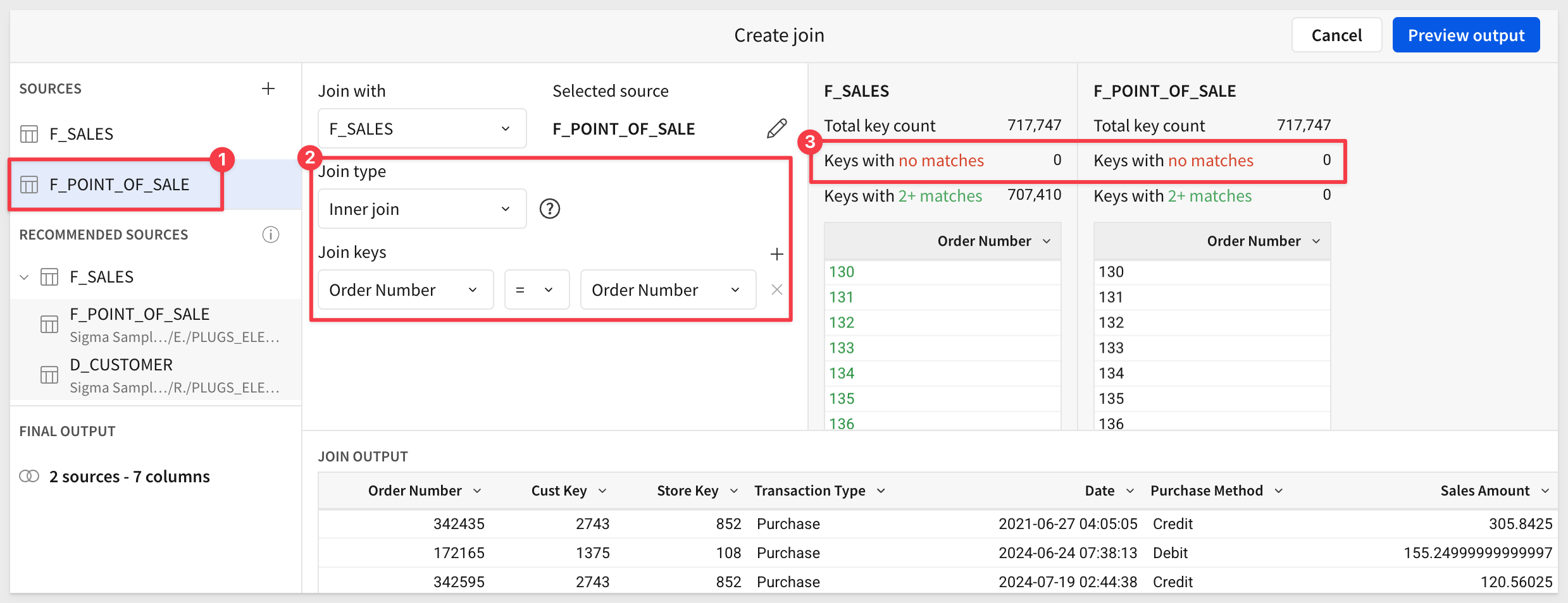
Now choose the type of join and identify the join keys (matching columns from each table).
Since we're joining the two tables on Order Number, we have a 100% match. This works because every sale must have an order number, so it exists in both tables.
For more information, see Join types
Click Preview output. Sigma shows the tables lineage. This allows us to see how our table was constructed, which columns are selected and more. We could also join more tables from here:
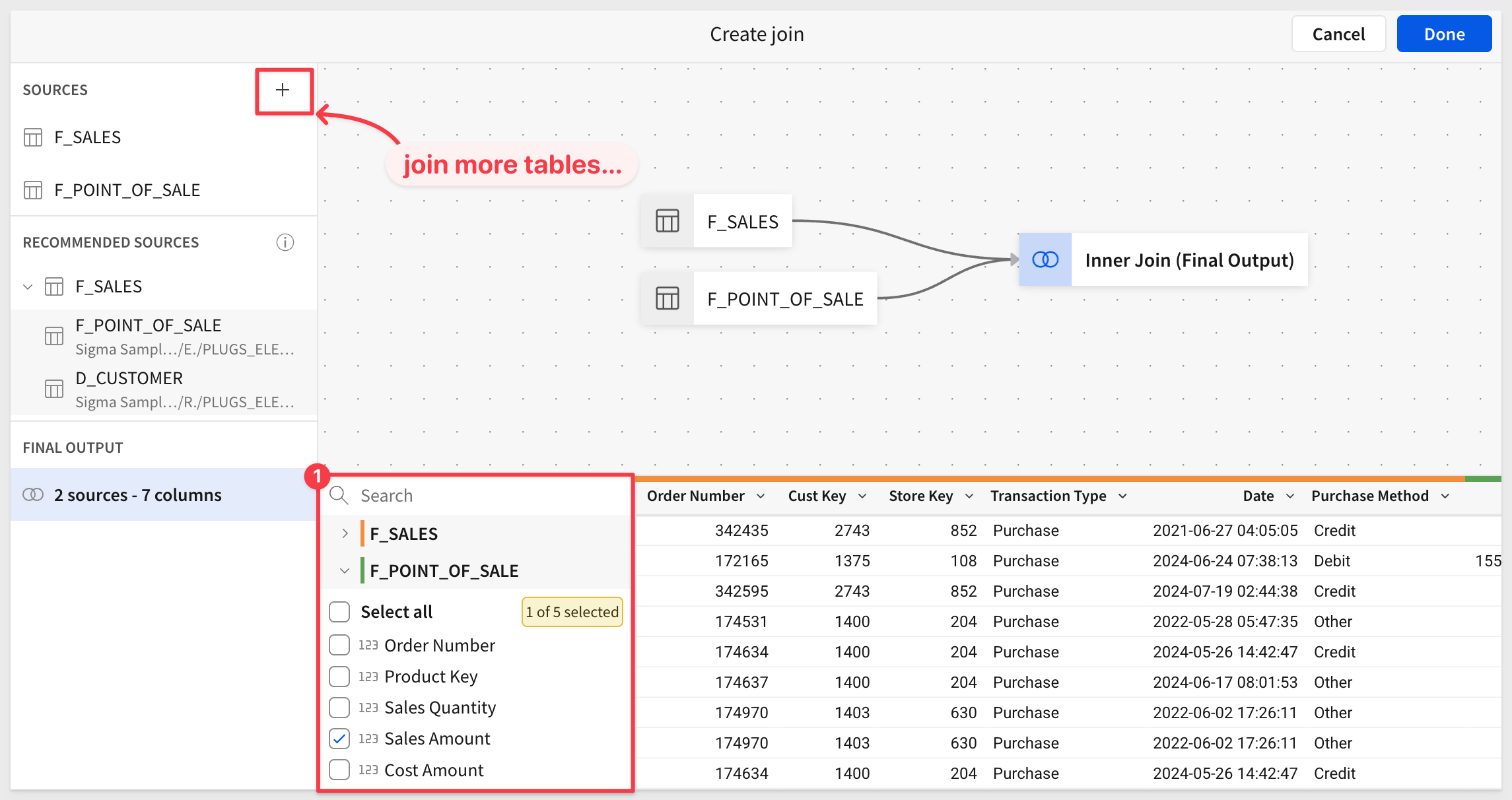
For more information, see View workbook and data model data lineage
Click Done, and rename the table Week_over_Week_Sales.
Drag the Date column to Groupings and truncate it to Week.
Hide the Order Number, Date and Sales Amount columns:
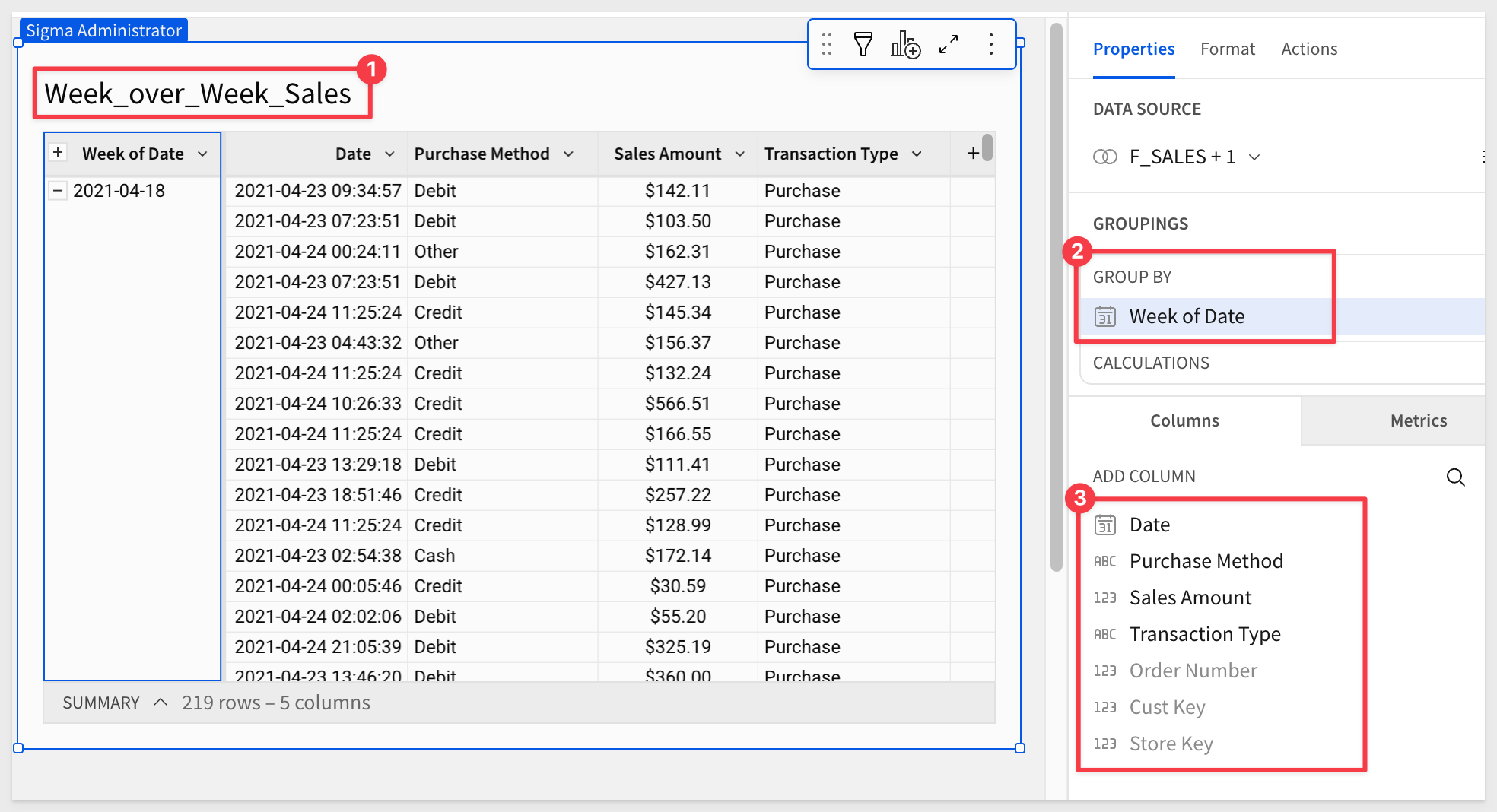
Drag the Sales Amount column to Calculations, rename it to Weekly_Sales and set the format to currency:
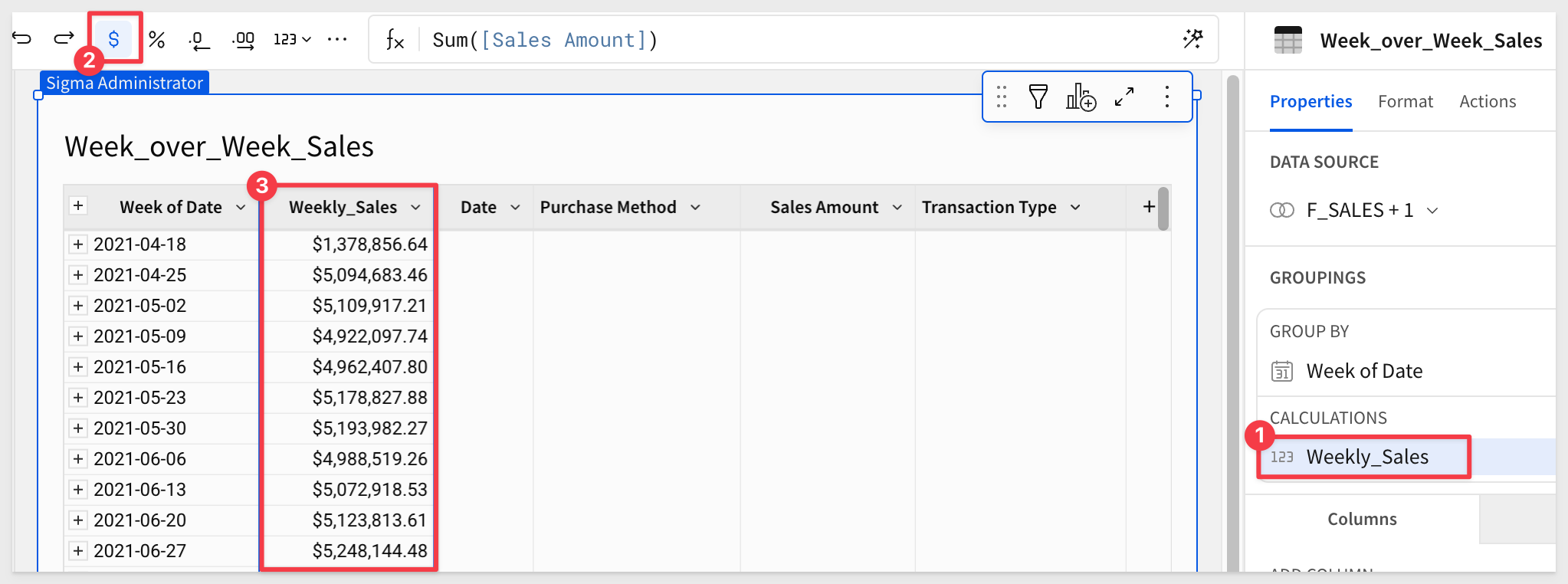
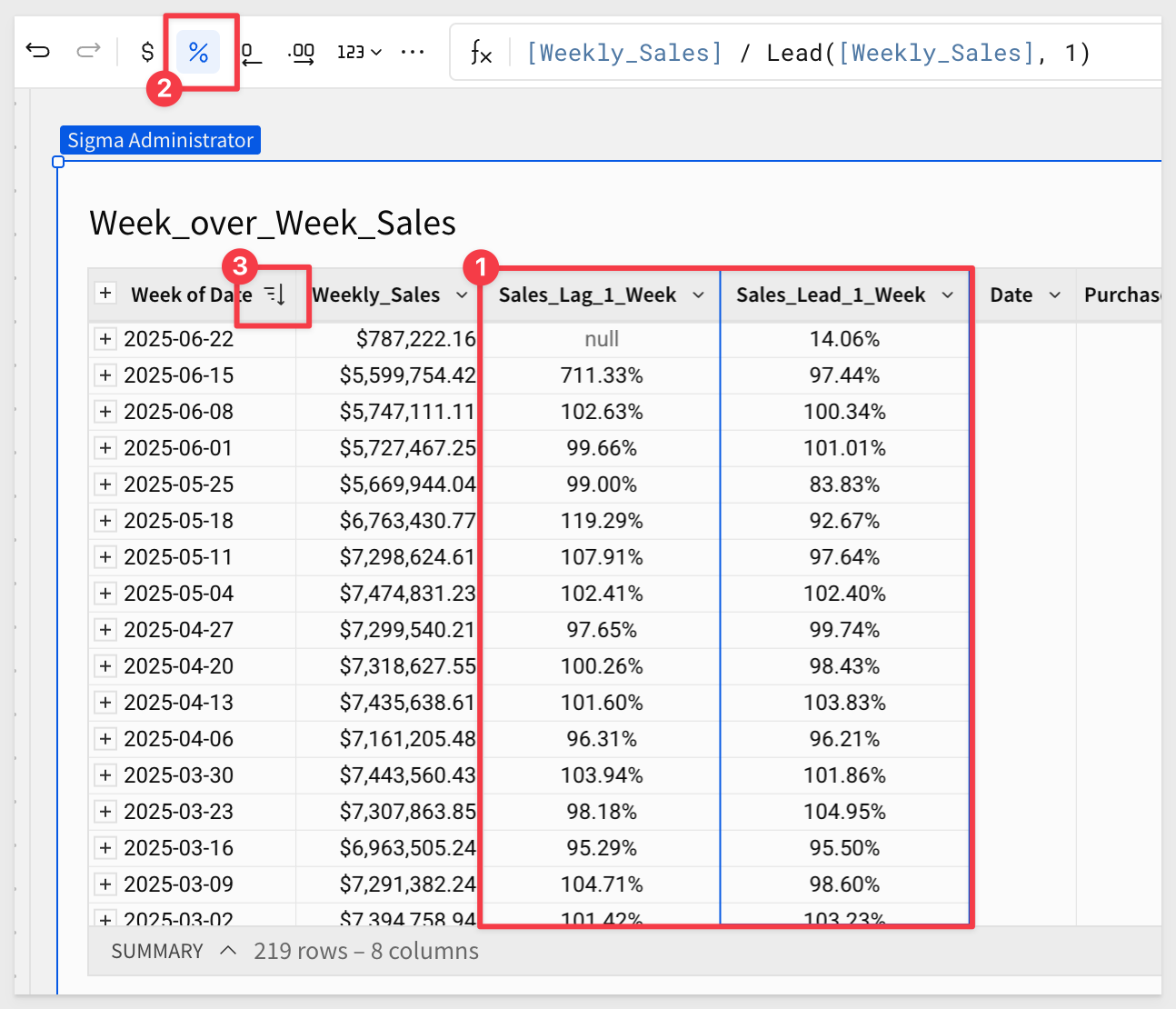
Add two calculated columns using the + icon in the CALCULATIONS panel. Rename each and set the formulas to:
Column:                         Formula:
Sales_Lag_1_Week      [Weekly_Sales] / Lag([Weekly_Sales], 1)
Sales_Lead_1_Week     [Weekly_Sales] / Lead([Weekly_Sales], 1)
Format the Lead/Lag columns as percentages and sort the Week of Date column in descending order:
For more information, see Lead
Sales Operations can now compare weekly sales performance at a glance.
This use case could also be solved using Sigma's DateLookback function. The DateLookback function returns the value of a variable at a previous point in time (or lookback period) determined by a specified date and offset.
We will use DateLookback in the next section.
Viewing data organized year over year by month helps users understand business performance in use cases like seasonality. It allows users to see whether performance is improving, flat, or declining year over year.
Now that we've learned how to navigate Sigma, we'll move a bit faster.
Since we'll reuse the Page 1 source, rename the page to Data.
Add a new workbook page and add another child of the PLUGS_ELECTRONICS_HANDS_ON_LAB_DATA table to it.
Rename the page Year over Year and the table to Year_Over_Year_by_Month.
Add the Today column back as we did in the last section.
Start by hiding all columns. Use Shift + Click to select the first and last, then click Hide column.
Now we have lots of columns to work with but none are displayed:
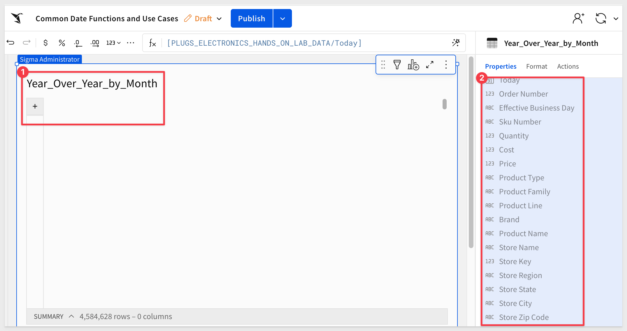
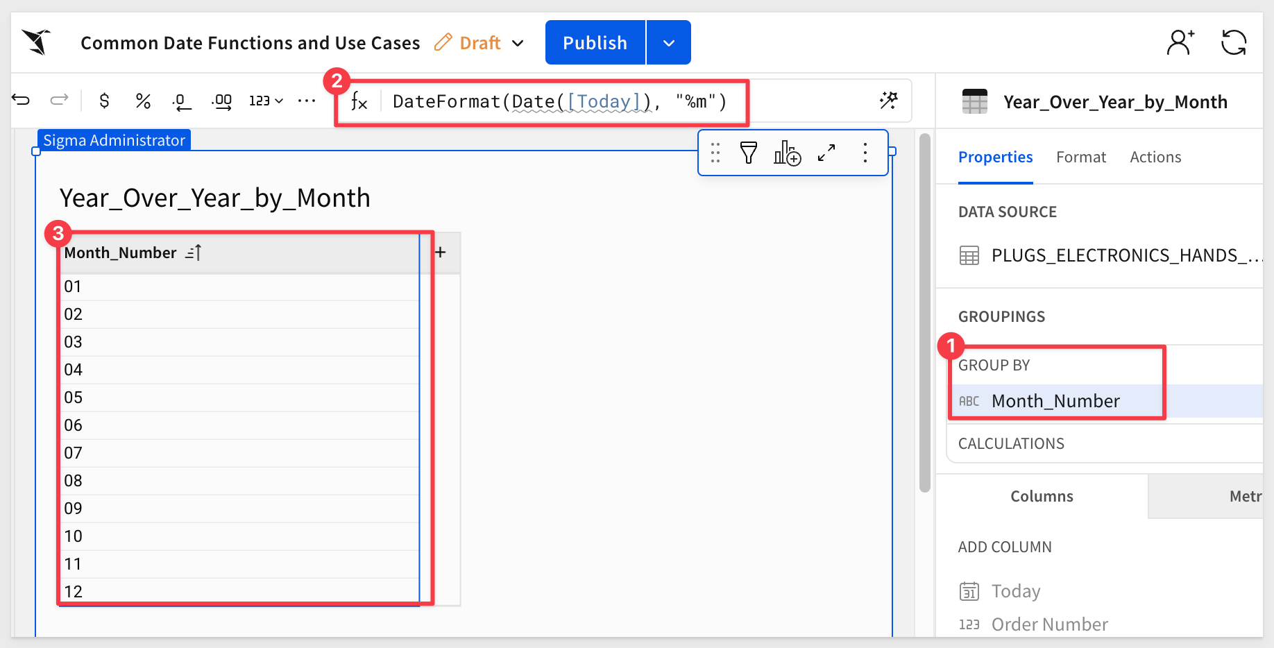
Add a new grouping by clicking the + next to GROUPINGS and selecting the Today column.
Set the formula for the Day of Today column to:
DateFormat(Date([Today]), "%m")
Rename this column Month_Number and set its sort order to Ascending.
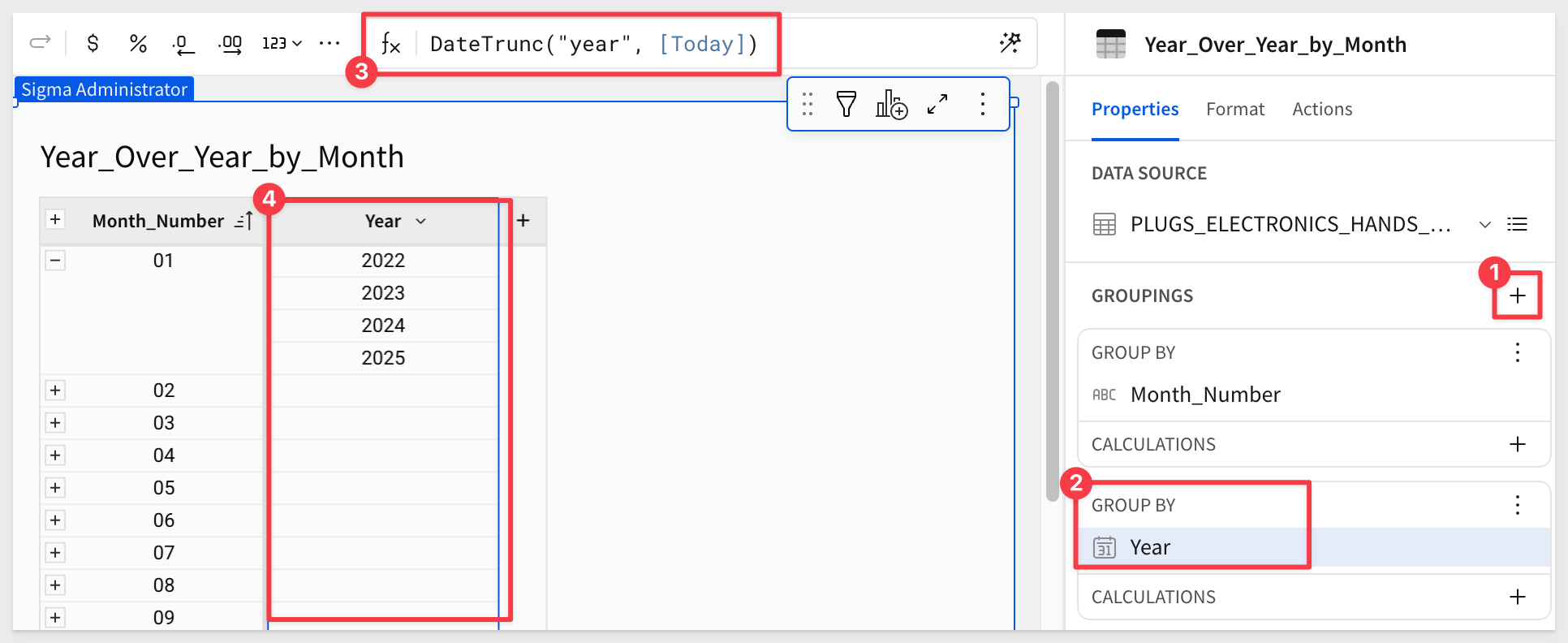
Add another GROUPING selecting the Today column again.
Set the new column's formula to:
DateTrunc("year", [Today])
Rename the column Year:
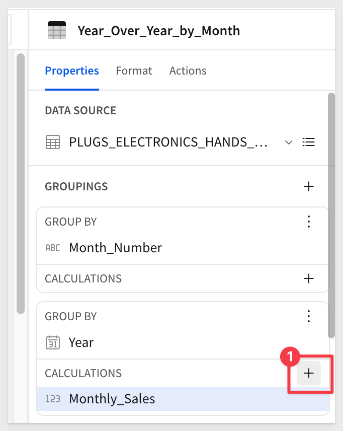
Add a new calculation by clicking the + next to CALCULATIONS in the Year grouping, and select New column:
Sum([Quantity] * [Price])
Format the column as currency.
The table should now look similar to this (after collapsing/expanding and formatting):
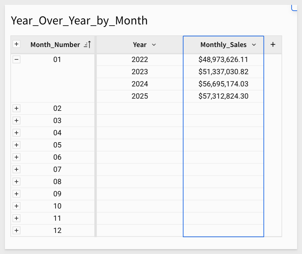
Add a new CALCULATION by clicking the + to the right of CALCULATIONS in the Year grouping and select New column.
Configure the new column as shown below:
Column Name:       Formula:
Previous_Year      DateLookback([Monthly_Sales], [Year], 1, "year")
Now we can calculate the year over year percentage difference for each month.
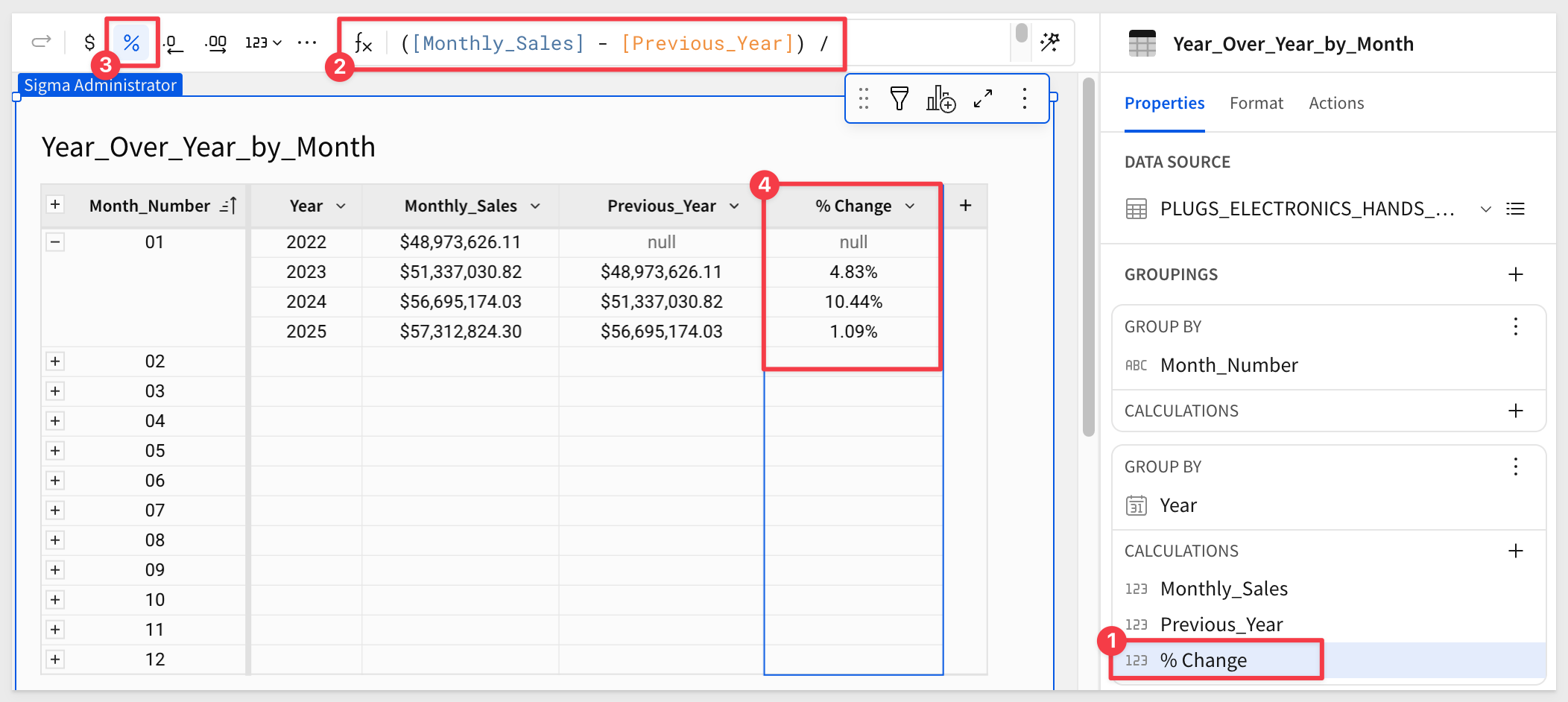
Add another new CALCULATION column to the same grouping and configure it using:
Column Name:      Formula:
% Change          ([Monthly_Sales] - [Previous_Year]) / [Previous_Year]
Set the column's format to Percentage.
Now we can start to see trends in the data.
For more information, see DateLookback
Click Publish.
The InDateRange function provides a succinct way to write calculations such as last year or this year. It also simplifies more complex calculations, making them shorter and easier to read. While there are other ways to solve this, let's explore a different approach using InDateRange.
What's differnt with the InDateRange function is that it will return True or False based on its configuration. The table can then be filtered based on an InDateRange column being True or False.
For example, we may want to see how sales this year compare with last year, side by side.
Create a new page and rename it to InDate Range.
Add another child of the PLUGS_ELECTRONICS_HANDS_ON_LAB_DATA table and move it to the new page.
Rename the table Sales_Comparison.
Add the Today column back to the table.
Add a new column using this configuration:
Column Name:      Formula:
Week              DatePart("week", [Today])
Add another new column using this configuration:
Column Name:      Formula:
Sales_Amount     [Price] * [Quantity]
Hide this column.
Next, use the InDateRange function to create four new columns.
For each of the following new columns, use the following configuration:
Column Name: Formula:
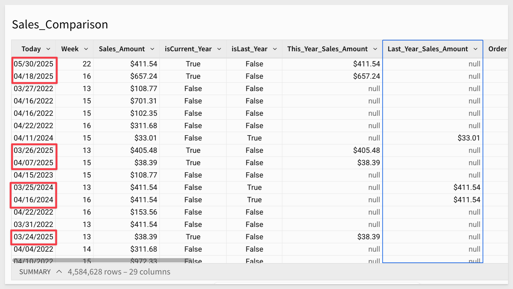
isCurrent_Year InDateRange([Today], "current", "year")
isLast_Year InDateRange([Today], "last", "year")
This_Year_Sales_Amount SumIf([Sales_Amount], [isCurrent_Year])
Last_Year_Sales_Amount SumIf([Sales_Amount], [isLast_Year])
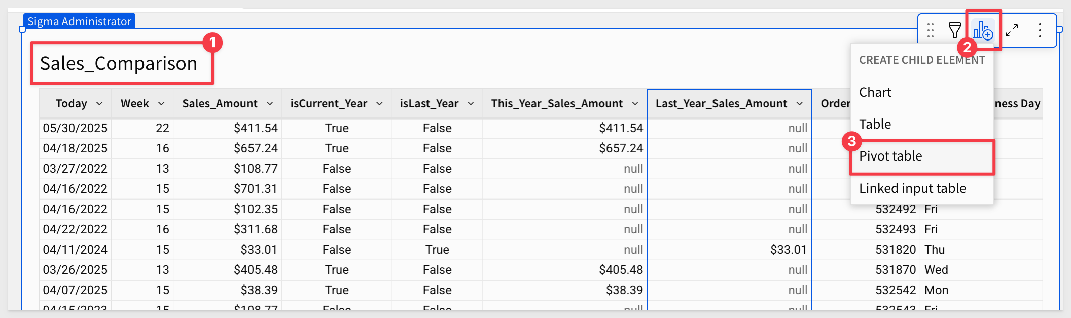
The table should now look like this. Notice that sales amount values only appear for the current and previous years. All others are null:
Instead of filtering the table to show only rows for the current and previous years, let's use a pivot table.
Add a child pivot table:
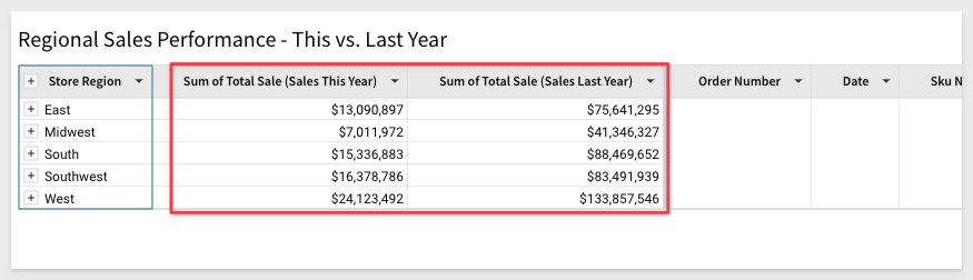
Configure the pivot table as shown below and rename it Sales - This Year vs. Last:
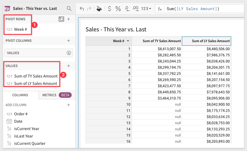
From here we can start to dig deeper into the analysis by calculating sales changes or adding visualizations.
For more information, see InDateRange
In this example, we'll demonstrate how to use data from one table in another using a Lookup.
Imagine two tables contain useful columns that are missing from a third table. To enrich the third table, we can use a Lookup to bring in those missing columns.
Lookups work by matching rows based on shared values between two columns—one from each table. These columns are known as join keys and we will simulate how this works using our existing sample data.
Add a new workbook page and place another child of the PLUGS_ELECTRONICS_HANDS_ON_LAB_DATA table from the Data page to it.
Another way to do this is to add a new Table from the Element bar and set the source as shown:
Rename the page Lookups and the table to Regional_Sales_Performance.
Add the Today column back as we did in the last section.
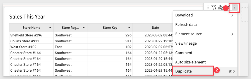
Duplicate the table using the table menu.
Rename this duplicated table Sales_This_Year
On the Sales_This_Year table, hide all the columns leaving only Store Name, Store Region, Store Key, and Today.
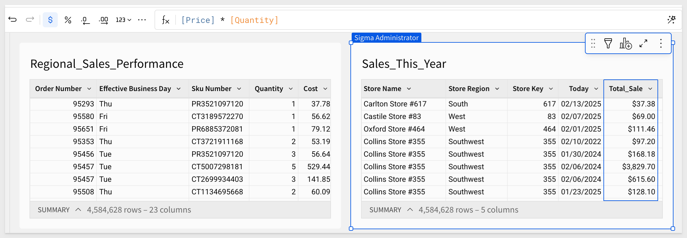
Add a new column, rename it Total_Sale and set its formula to:
[Price] * [Quantity]
Your page should now look like this:
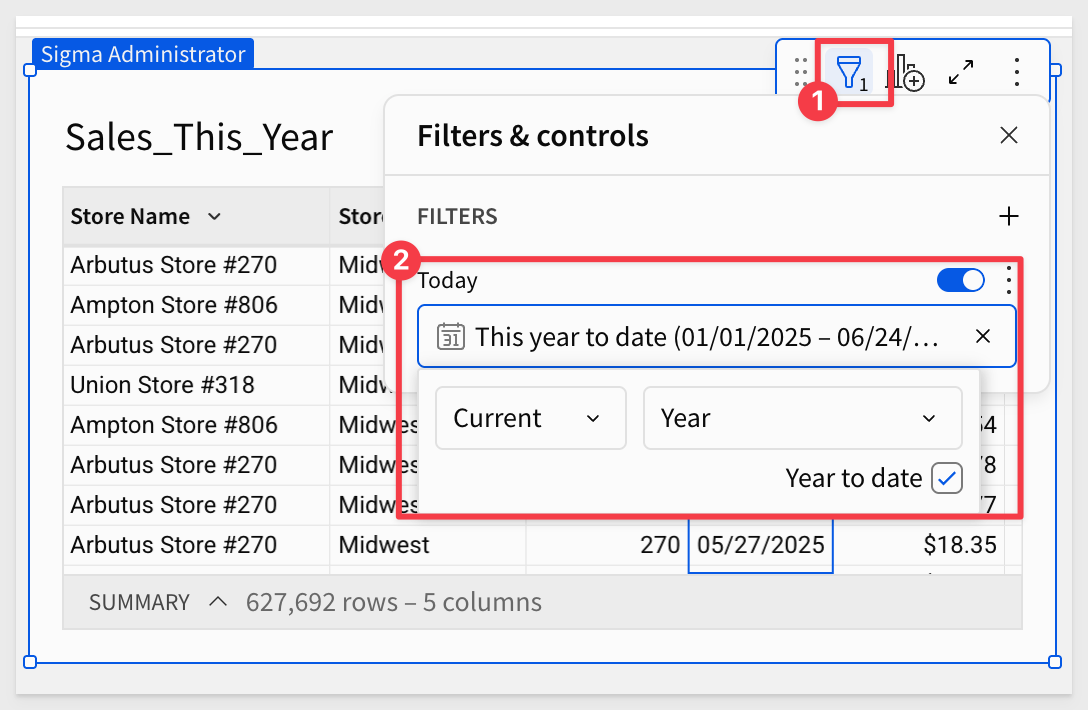
Filter this table to show only orders from this year (click the drop-down arrow on the Today column and select Filter):
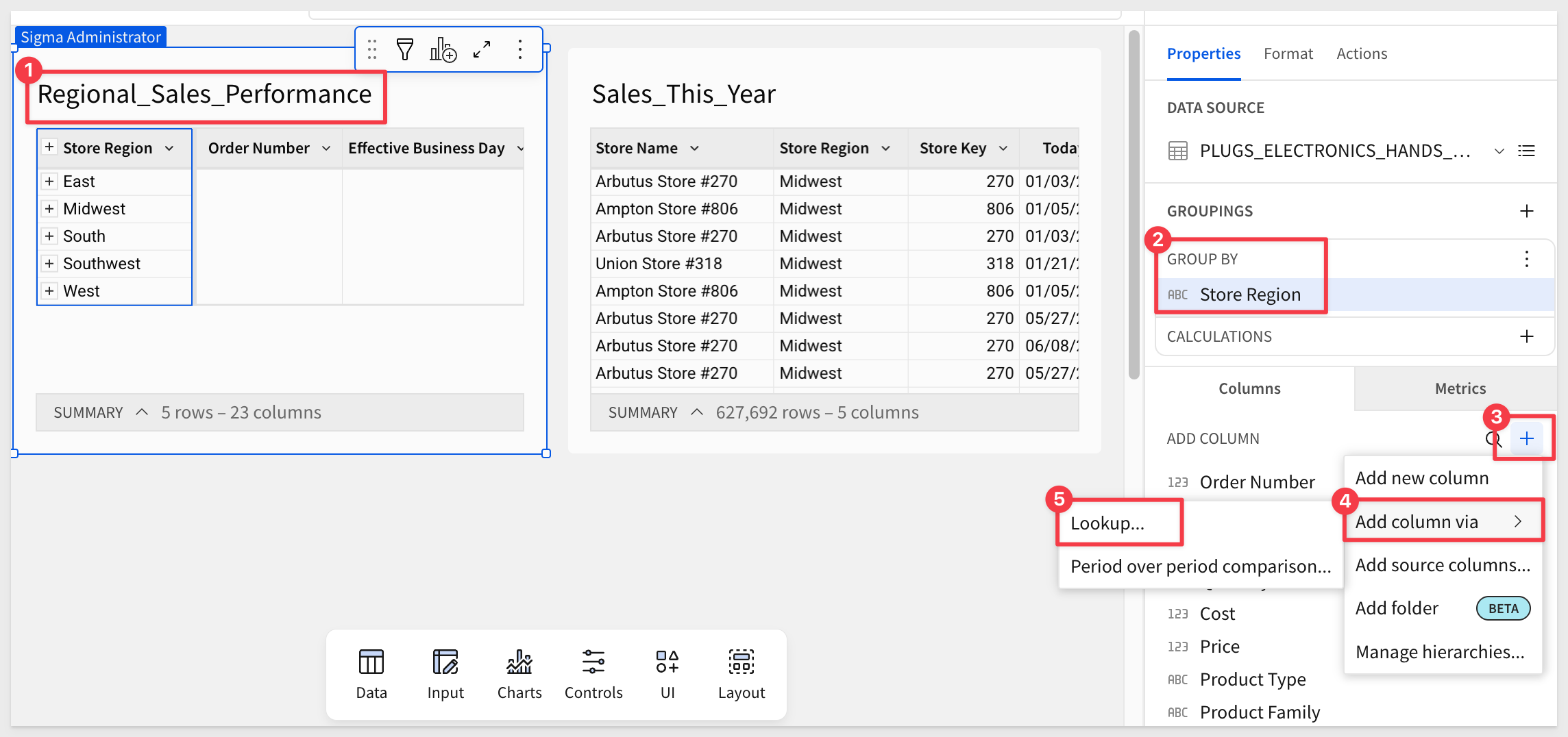
On the Regional Sales Performance table, we want to group on the Store Region column.
Now add a new column via lookup:
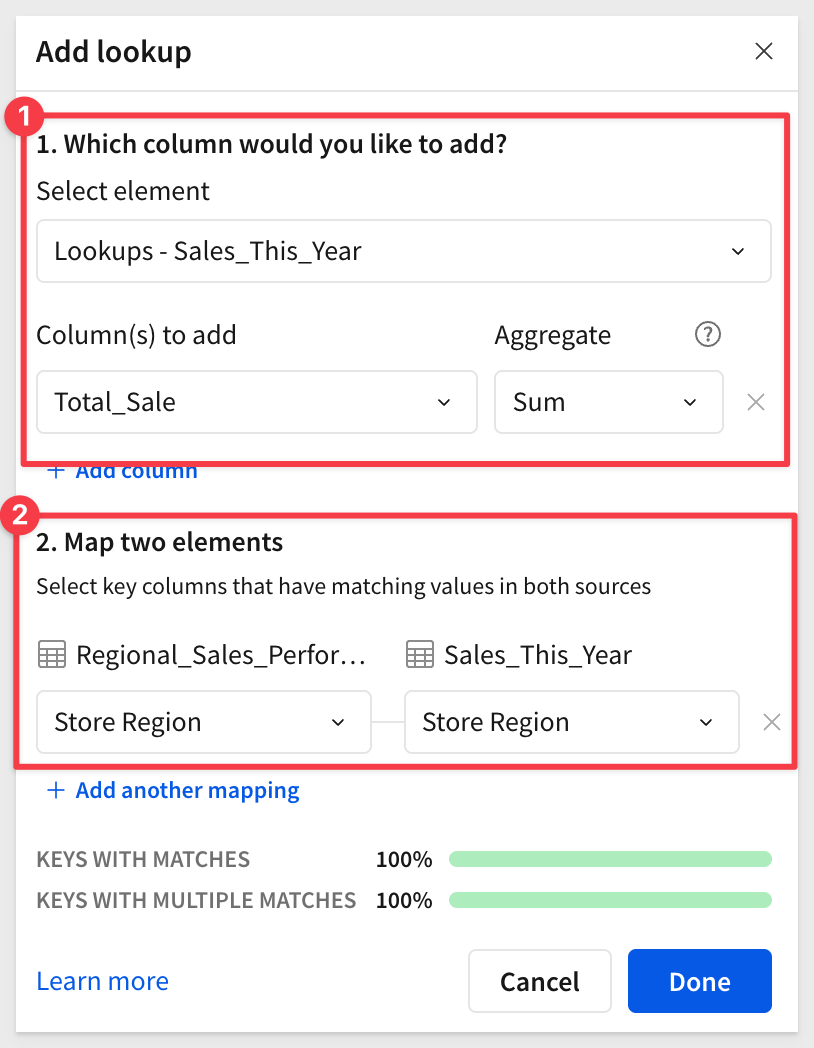
You will be prompted to set how the two tables will be joined. Use this configuration:
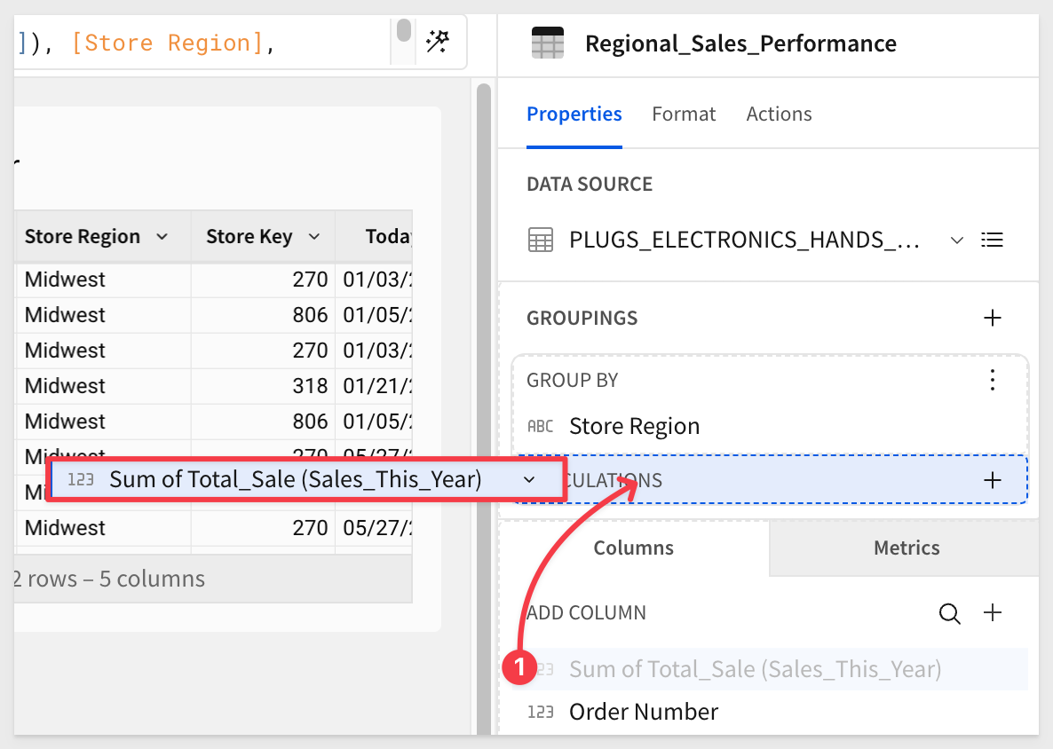
Now drag the new lookup column to the Calculations section of the Store Region grouping:
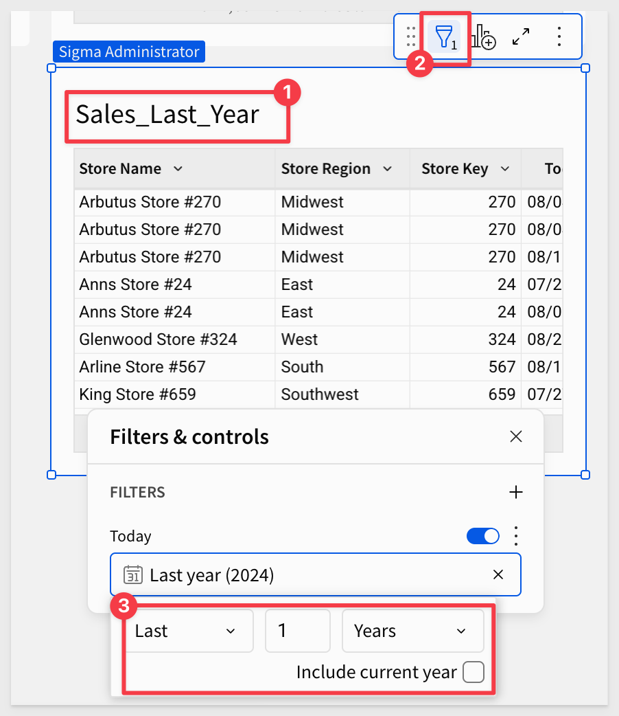
Now let's get last year's sales. Duplicate the Sales_This_Year table:
Rename the table to Sales_Last_Year.
Change the filter to use last year as the range:
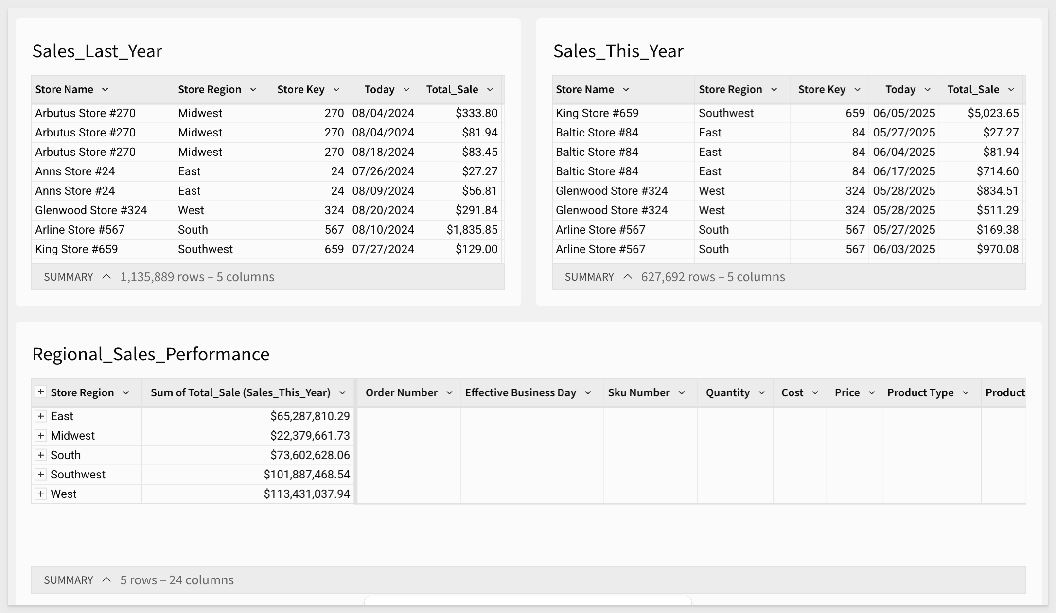
The page should now look like this (after rearranging elements as needed):
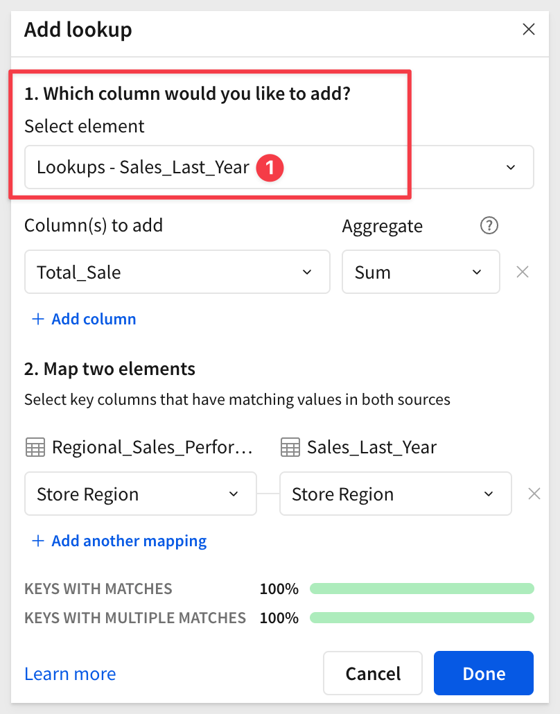
Now add another lookup column to the Regional_Sales_Performance table, using Sales_Last_Year as the source.
The only configuration difference is the source table as shown:
Drag this new column into the Calculations section—and we're done. We now have both last year's and this year's sales by store region, with full detail.
For more information, see Add columns through Lookup
The InPriorDateRange function is used to calculate values from a prior time period such as "This Week Last Year".
It returns a Boolean (True or False), which we can use to filter rows.
To speed things up, duplicate the Lookups page and rename the copy InPrior_Date_Range.
Rename the Sales_This_Year table to Sales_In_Current_Quarter.
Also rename the Sales_Last_Year table to Sales_Last_Year_Same_Quarter.
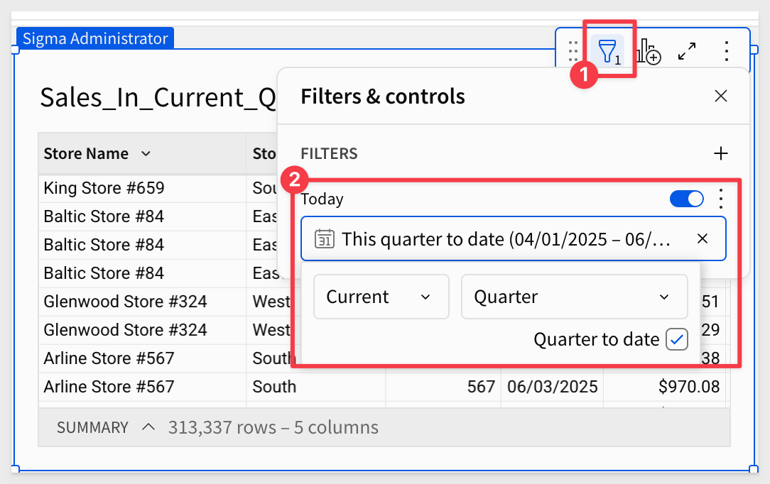
In the Sales_Last_Year_Same_Quarter table, we want to filter the data to show only the rows from last quarter. We can do that by simply using the filters control:
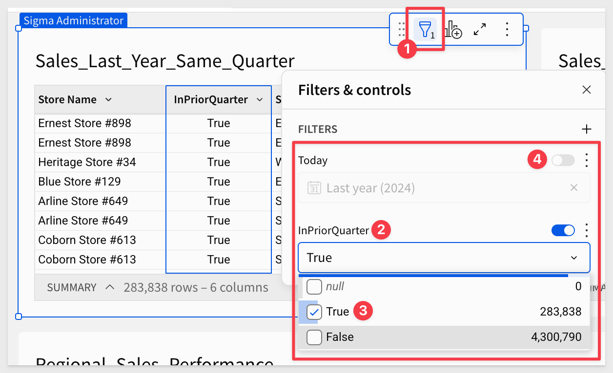
In the Sales_Last_Year_Same_Quarter, add a new column named InPriorQuarter and set its formula to:
InPriorDateRange([Today], "quarter", "year")
This will evaluate the Today column and return true or false if the date is in the quarter, one year prior.
Next, update the table's filters by adding a new one on the InPriorQuarter column and set it to show only rows where the value is True.
We can disable the filter for Today since our formula is providing the filter now:
Since the Regional_Sales_Performance table already uses lookups to bring in the Total Sale column from both source tables, we don't have to do anything; the sales are summed and grouped already.
We are done:
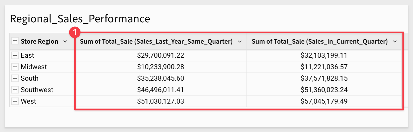
Compare these values to those on the Lookups page—you'll see they are significantly lower.
Companies often use table-based calendars in analytics to help address data consistency, seasonality, and planning.
In this QuickStart step, we'll build a pivot table that leverages the NRF Retail 4-5-4 Calendar combined with our Plugs Electronics sample data to analyze same-store sales the way most retailers prefer. These same general methods apply to any table-based calendar you use.
The NRF Retail 4-5-4 Calendar is a standardized retail calendar developed by the National Retail Federation (NRF) to help retailers track and analyze their sales performance. It is widely used by retailers in the United States, and it is particularly useful for businesses that operate on a fiscal year that does not align with the traditional calendar year. The calendar helps retailers plan their inventory, staffing, and marketing strategies based on historical sales data and seasonal trends.
For more information, see NRF 4-5-4 Calendar
Add a new workbook page, and this time, add the PLUGS_ELECTRONICS_HANDS_ON_LAB_DATA table by selecting it from the sample database instead of the Data page:
Rename the page Date_Calendar.
Rename the table to Same_Store_Sales.
Add a new column, rename it to Order_Value and use this formula:
[Quantity] * [Price]
Create a new join:
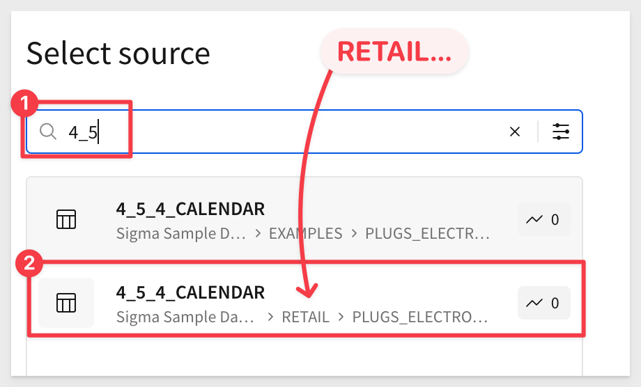
Search for the 4_5_4_CALENDAR in the RETAIL schema and select it:
We are now presented with a screen that allows us to adjust how the two tables are joined. We need to adjust the join to use the Date and Today columns
If we look closely at the join results we can see there is a mismatch; the timestamps are causing a problem:
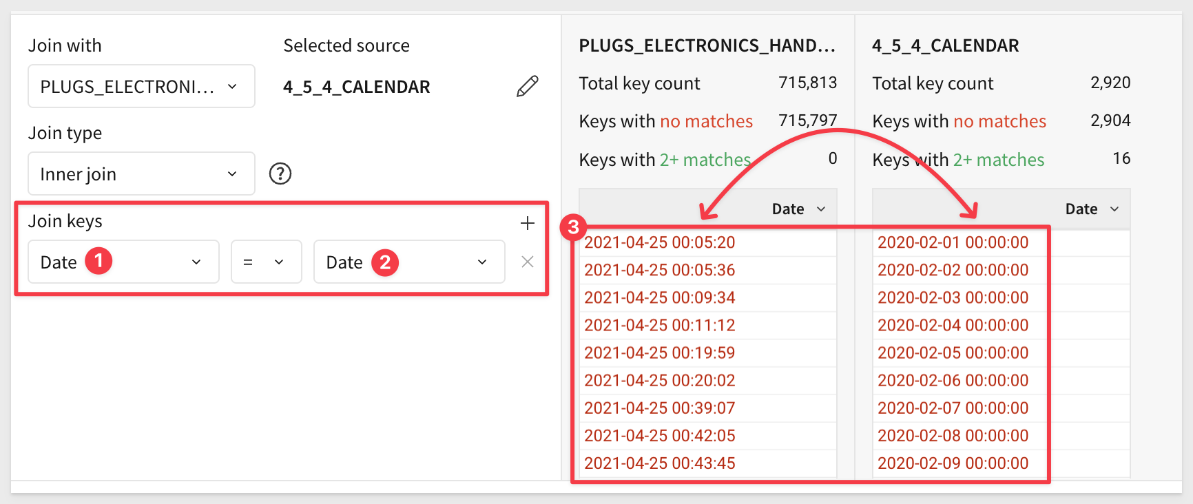
Joining on mismatched data types can cause issues, but Sigma supports formula-based joins to correct the issue.
To handle the datatype issue, we will use a formula for each join key:
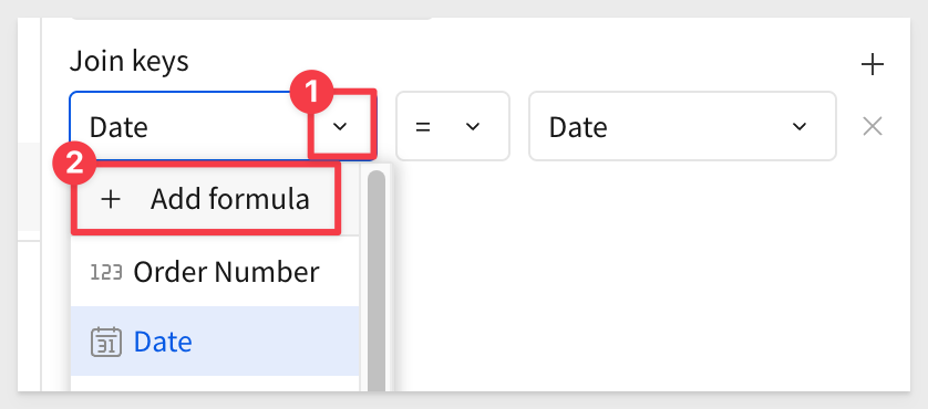
Apply this formula to both join keys:
DateTrunc("day", [DATE])
After making the changes, you should have many matches. It won't be a 100% match, as some values in the Plugs table that are not in the 4-5-4 table.
Click Preview Output and Done.
Now, create a child of this table and select Pivot Table as the type:
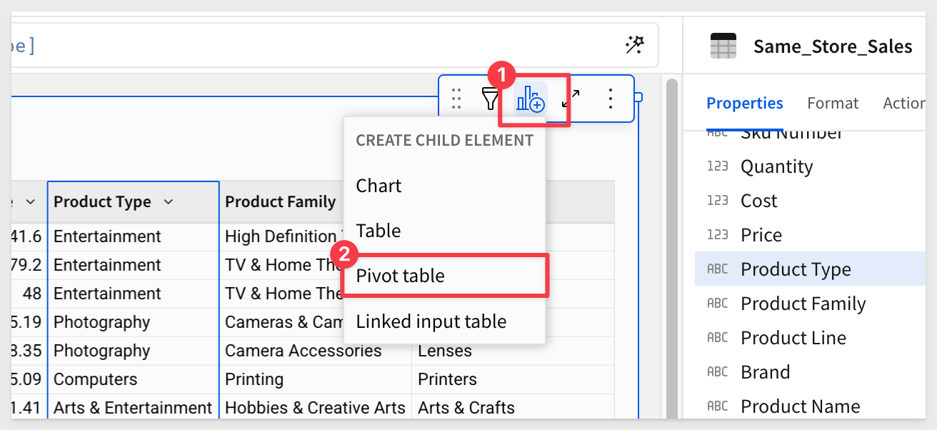
Rename the pivot table to Same_Store_Sales_454_Calendar.
Configure the pivot table as shown below:
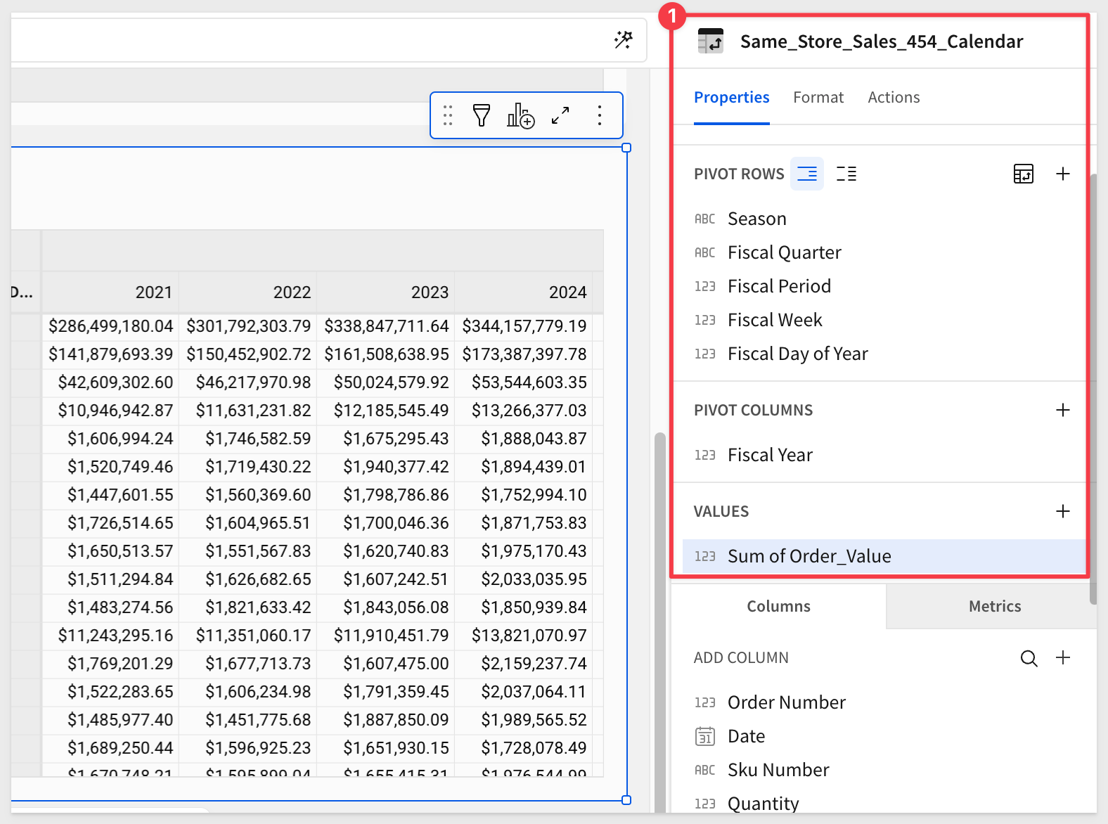
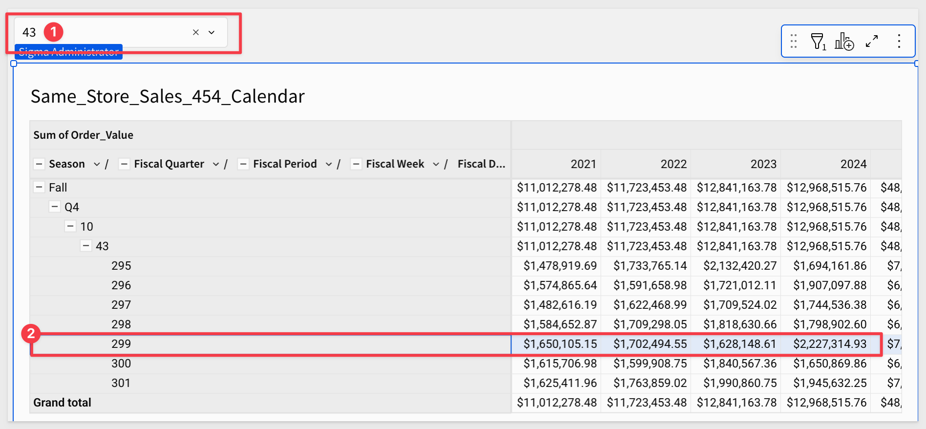
Let's say we want to see same-store sales for Thanksgiving. The Fiscal Day of the Year value according to the 4-5-4 Calendar is 299 in week 43.
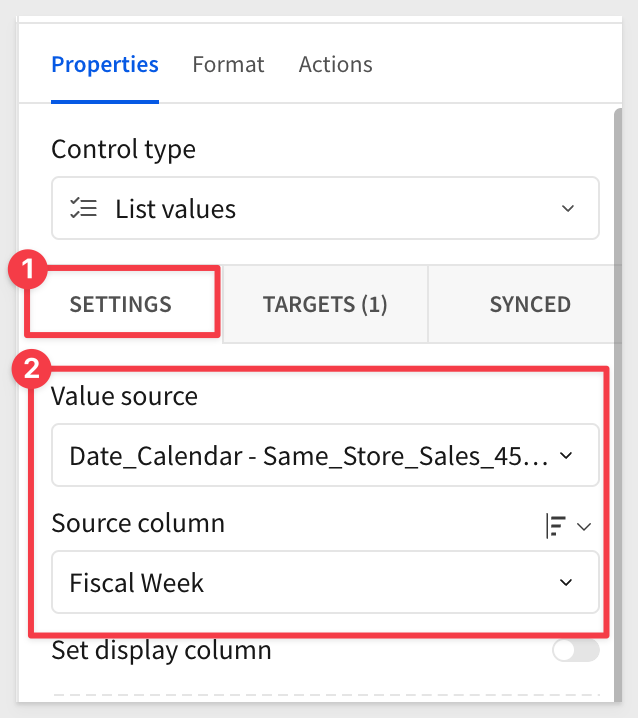
We can add a list page control to the page:
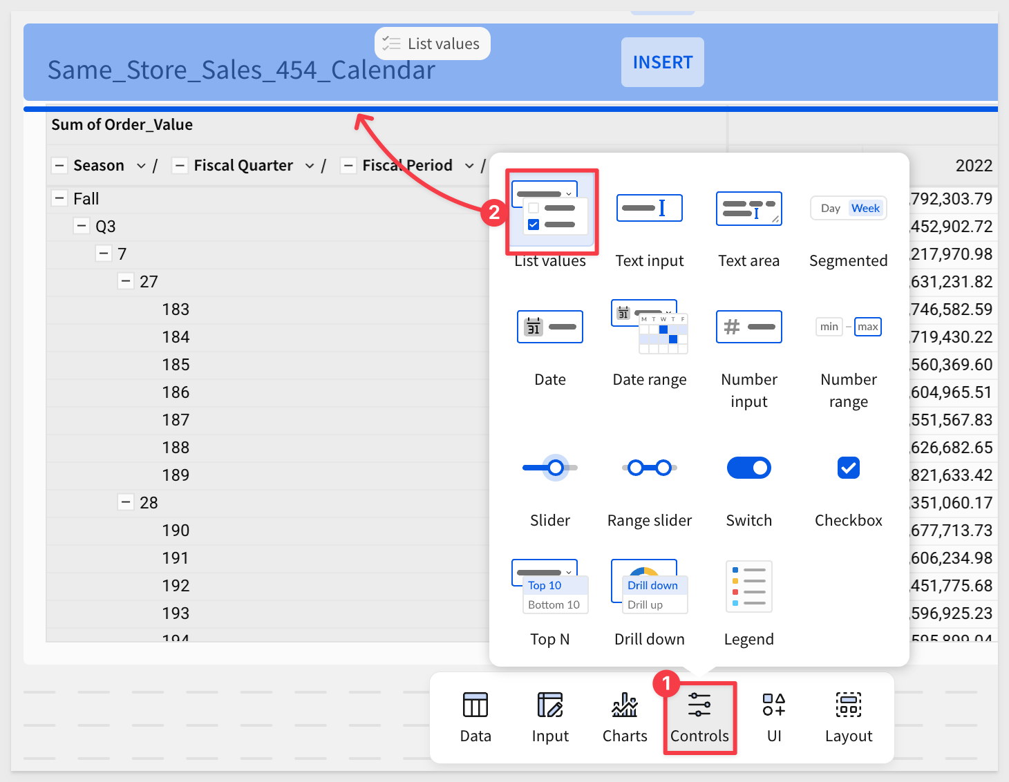
Configure it to filter based on the Fiscal Week:
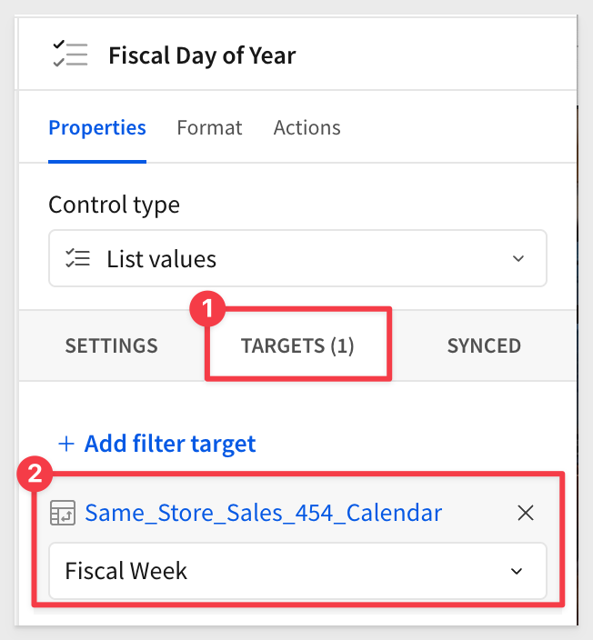
And set its target to Fiscal Week:
Use the control to find week 43:
Click Publish.
Of course, we could make this more user-friendly by making a control that shows major holidays by name and other improvements but that is outside the scope of this QuickStart.
In this QuickStart, we explored many of the most commonly used date functions and the use cases where they're applied. While not comprehensive, this guide highlights key patterns and techniques for working with dates in Sigma. There are many more ways to leverage dates—so keep exploring!
For more information, see Function index
Additional Resources:
Be sure to check out all the latest developments at Sigma's First Friday Feature page!
Blog
Community
Help Center
QuickStarts