Sigma provides over 200 functions that enable you to transform, calculate, and analyze data directly in your workbooks.
This QuickStart focuses on some of the most frequently used functions, demonstrating practical applications through hands-on examples using sample retail data.
You'll learn how to categorize values, handle null data, filter and search text, enrich datasets with lookups, calculate percentages, parse patterns, analyze hierarchies, and implement conditional logic—all essential skills for building powerful analytics in Sigma.
Template
We have also made the final workbook that is created during this QuickStart available as a Sigma Template. This option allows you to read along while having the workbook built for you. The template is not required and the end result is the same if you build it yourself.
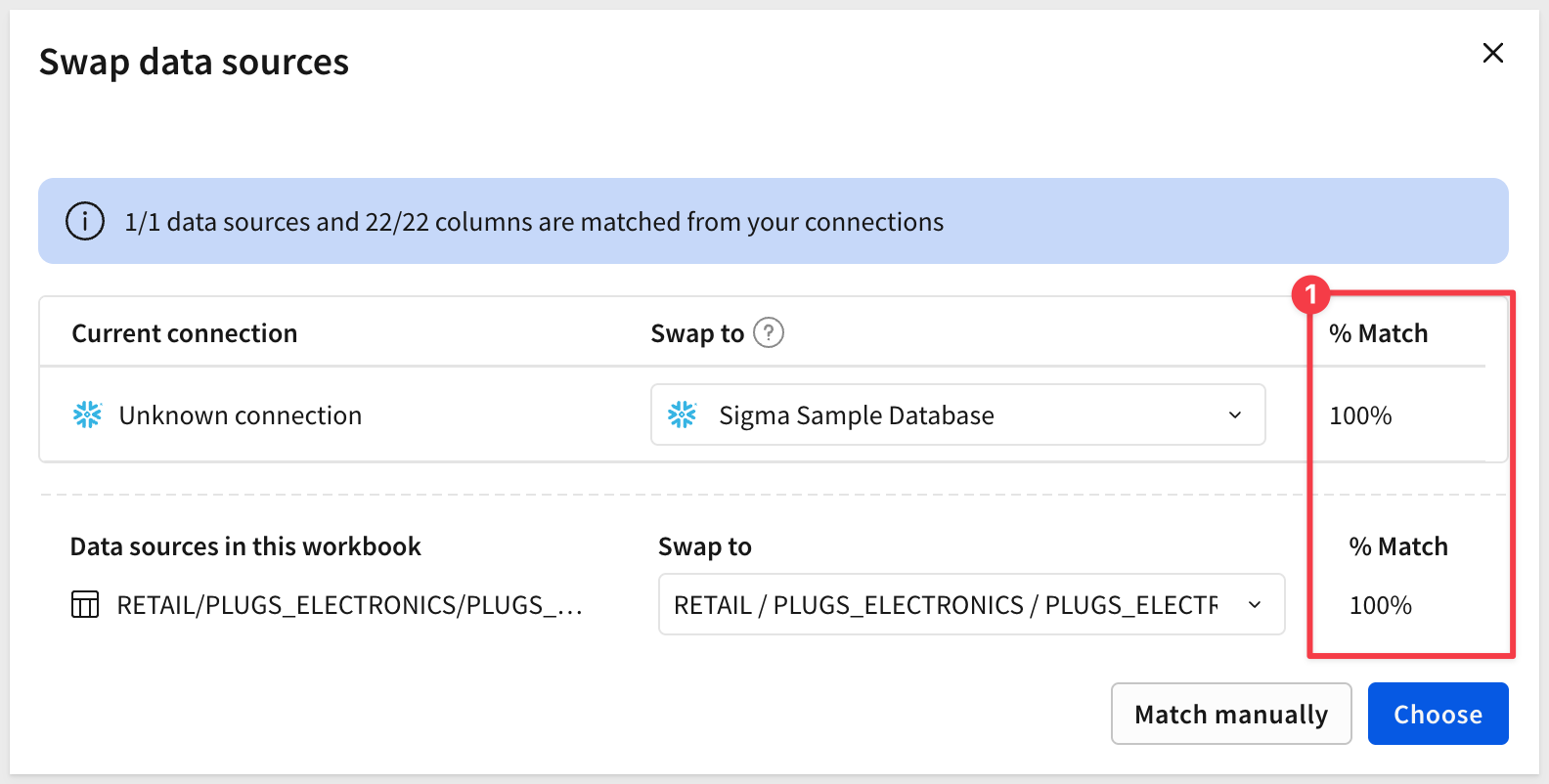
The template will prompt to Swap data sources. Since it uses Sigma provided sample data, the % Match should be 100%.
Click Choose:
Once done, the fully-built workbook is presented and we can Accept the swap and save the workbook normally:
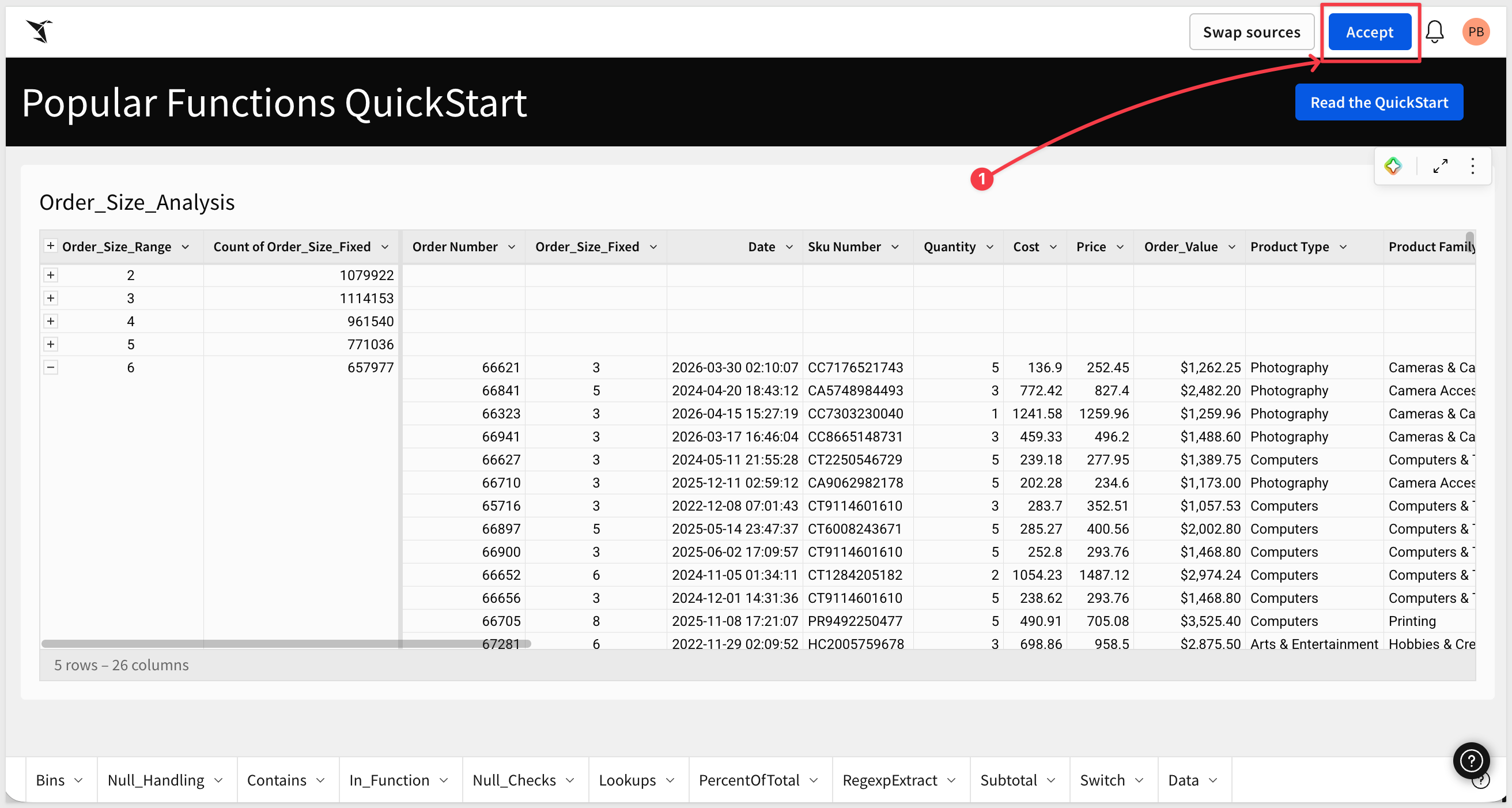
Save the workbook as Popular Functions QuickStart.
For more information on Sigma's product release strategy, see Sigma product releases
If something doesn't work as expected, here's how to contact Sigma support
Target Audience
The typical audience for this QuickStart includes users of Excel, common Business Intelligence or Reporting tools, and semi-technical users who want to try out or learn Sigma.
Prerequisites
- Any modern browser is acceptable.
- Access to your Sigma environment.
- Some familiarity with Sigma is assumed. Not all steps will be shown, as the basics are assumed to be understood.

Log into Sigma, click Create new and select Workbook.
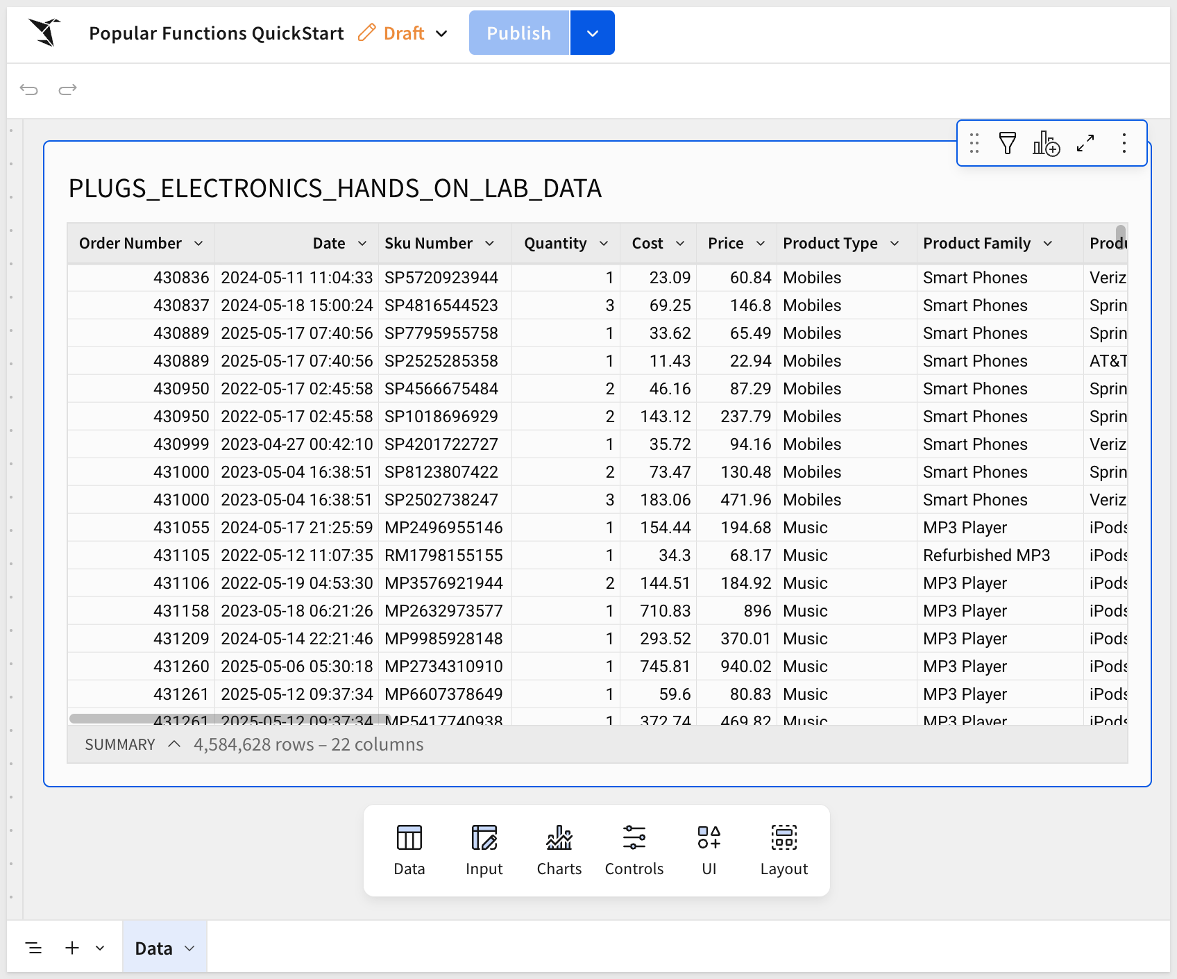
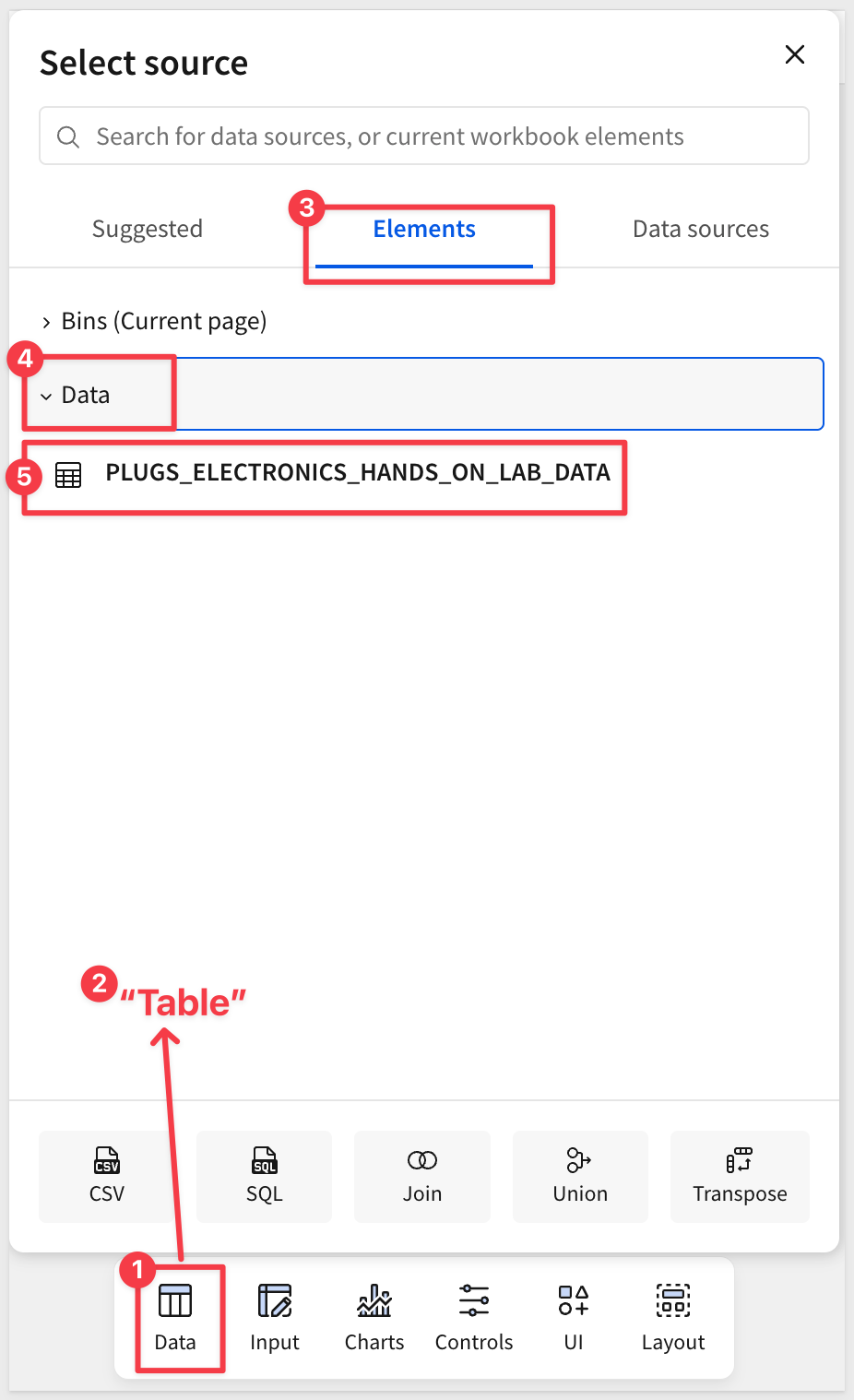
From the Element bar, under the Data group, place a new Table on the page.
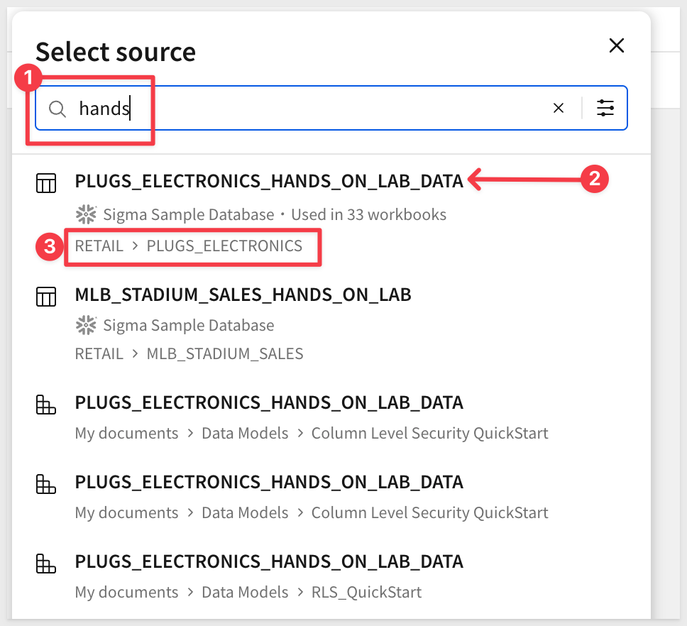
In the Select source modal, search for Hands and select the PLUGS_ELECTRONICS_HANDS_ON_LAB_DATA table from the RETAIL database:
Rename the page Data.
We will use this table multiple times by creating child tables from it to use on other pages.
Save the workbook as Popular Functions QuickStart:
The BinFixed and BinRange functions allow you to group numeric data into categories or "bins" for easier analysis.
A common use case is analyzing order values by size to understand purchasing patterns and inform business decisions like pricing tiers or shipping policies.
Before we start analyzing bins, let's add a calculated column to our source table on the Data page so it's available to all child tables.
Navigate back to the Data page and add a new column to the PLUGS_ELECTRONICS_HANDS_ON_LAB_DATA table:
Column Name:     Formula:
Order_Value      [Price] * [Quantity]
Format as currency.
Now create a new page and rename it to Bins.
Add a child table from the Data page's PLUGS_ELECTRONICS_HANDS_ON_LAB_DATA table:
Rename the table to Order_Size_Analysis.
Notice that the Order_Value column is now available in this child table.
BinFixed
BinFixed creates equal-width bins by dividing a range into a specified number of bins. This is useful when you want consistent bin sizes.
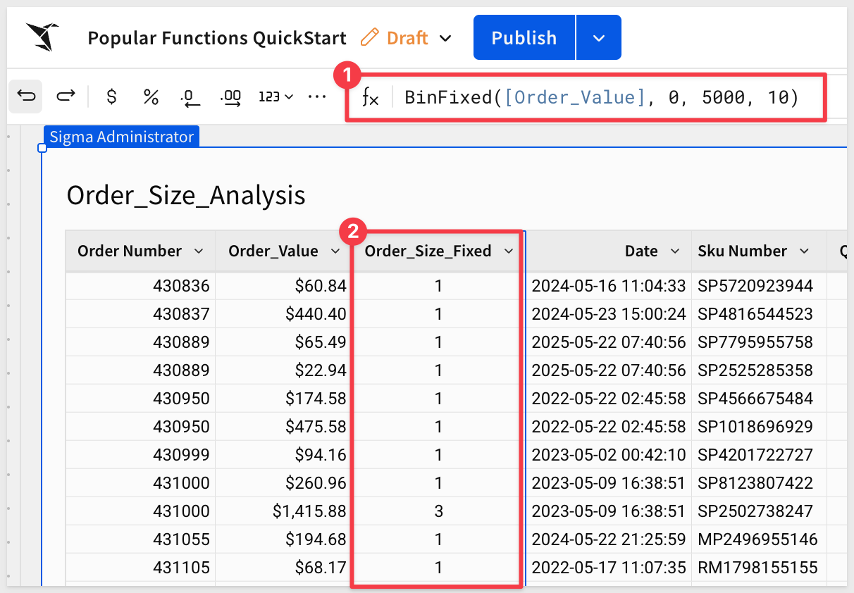
Let's group orders from $0 to $1000 into 10 equal bins. Add a new column:
Column Name:     Formula:
Order_Size_Fixed BinFixed([Order_Value], 0, 5000, 10)
This creates 10 equal bins of $500 each: "0-500", "500-1000", "1000-1500", etc.
Format the column as Number and remove the decimal places.
BinRange
BinRange allows you to define custom ranges that make business sense. This is useful when bin sizes should vary based on your analysis needs.
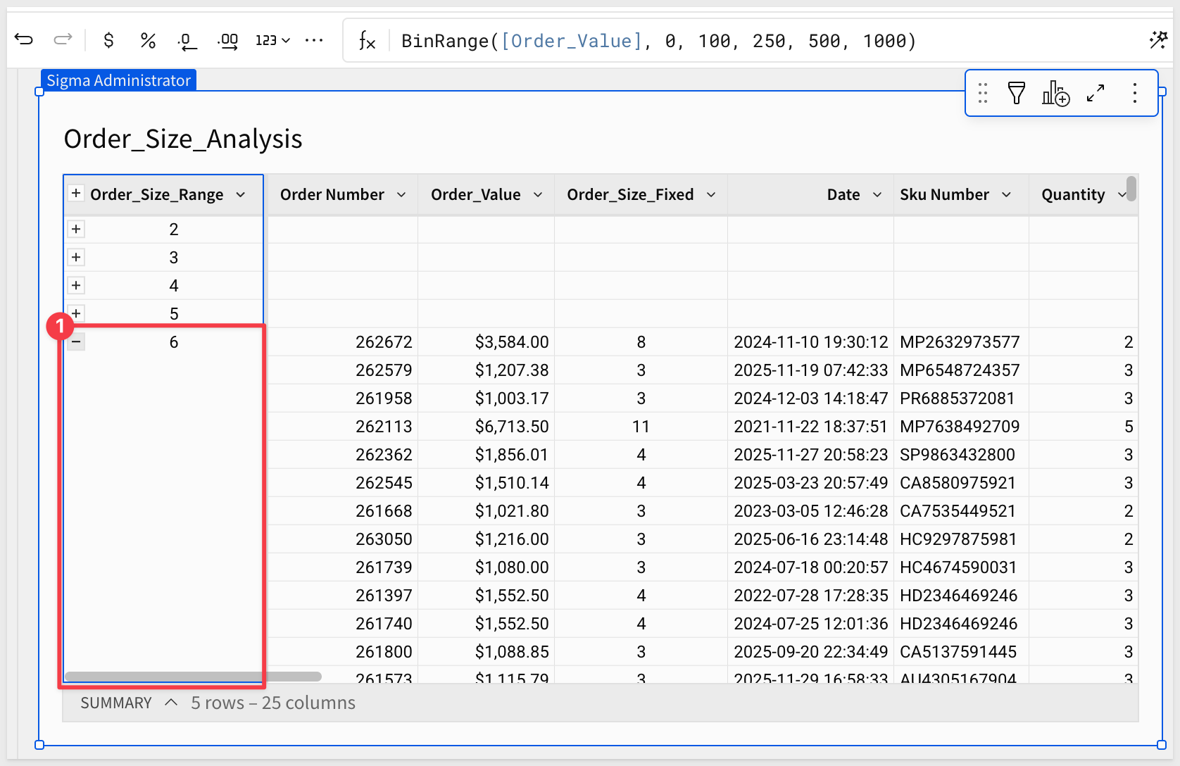
Add another new column:
Column Name:     Formula:
Order_Size_Range BinRange([Order_Value], 0, 100, 250, 500, 1000)
This creates bins:
- Small: $0-$100
- Medium: $100-$250
- Large: $250-$500
- Extra Large: $500-$1000
- Premium: $1000+
Now let's see the distribution. Group by Order_Size_Range and add a count:
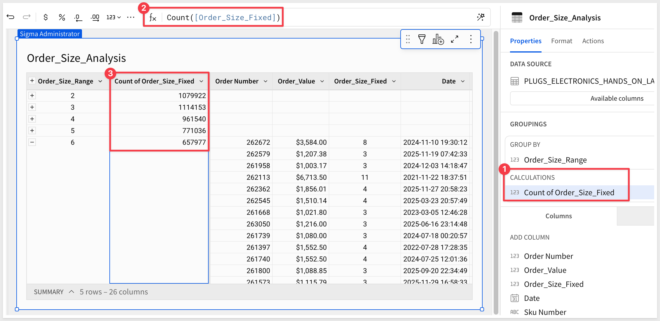
This shows most orders fall in the Small to Medium range, which could inform decisions about:
- Free shipping thresholds
- Volume discount tiers
- Inventory planning
For more information, see BinFixed and BinRange
Click Publish.
The Zn and Coalesce functions help handle null values in your data, which is essential for accurate calculations and clean reporting.
Use case: Calculate accurate commission rates and sales metrics even when some fields contain null values.
Create a new page and rename it to Null_Handling.
Add a child table from the Data page's PLUGS_ELECTRONICS_HANDS_ON_LAB_DATA table.
Rename the table to Sales_With_Nulls.
Notice that the Order_Value column is now available in this child table without needing to recalculate it.
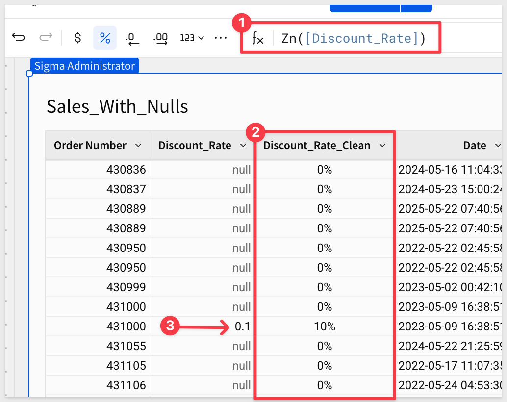
Zn()
Zn (Zero if Null) replaces null values with 0. This is the most common use case for handling nulls in numeric calculations.
Let's simulate a discount column that might have nulls. Add a new column:
Column Name:     Formula:
Discount_Rate    If([Order_Value] > 500, 0.10, null)
This gives a 10% discount only for orders over $500, otherwise null.
Now create a column that handles the null values:
Column Name:           Formula:
Discount_Rate_Clean    Zn([Discount_Rate])
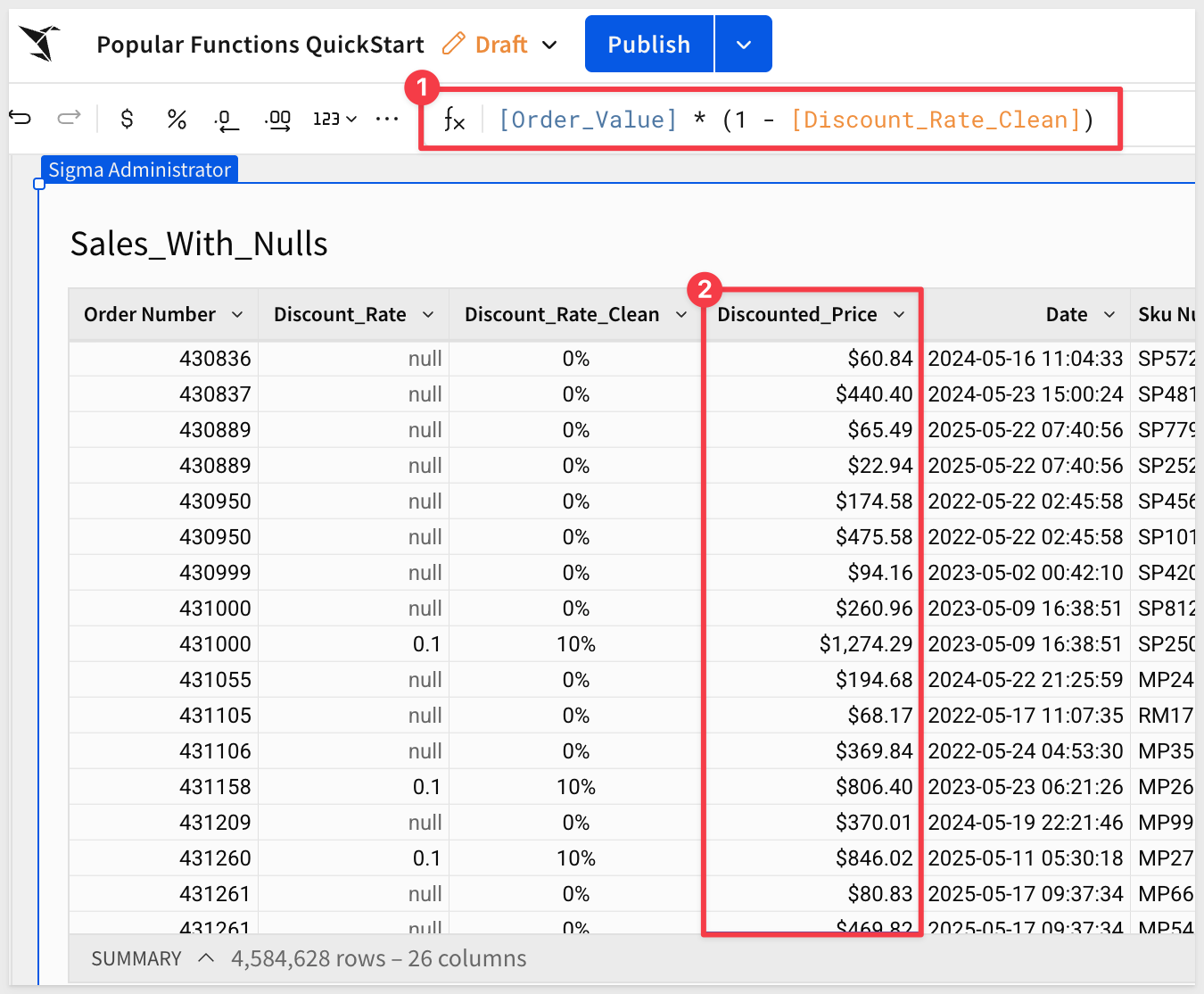
Now you can safely calculate discounted prices without worrying about null errors:
Column Name:         Formula:
Discounted_Price     [Order_Value] * (1 - [Discount_Rate_Clean])
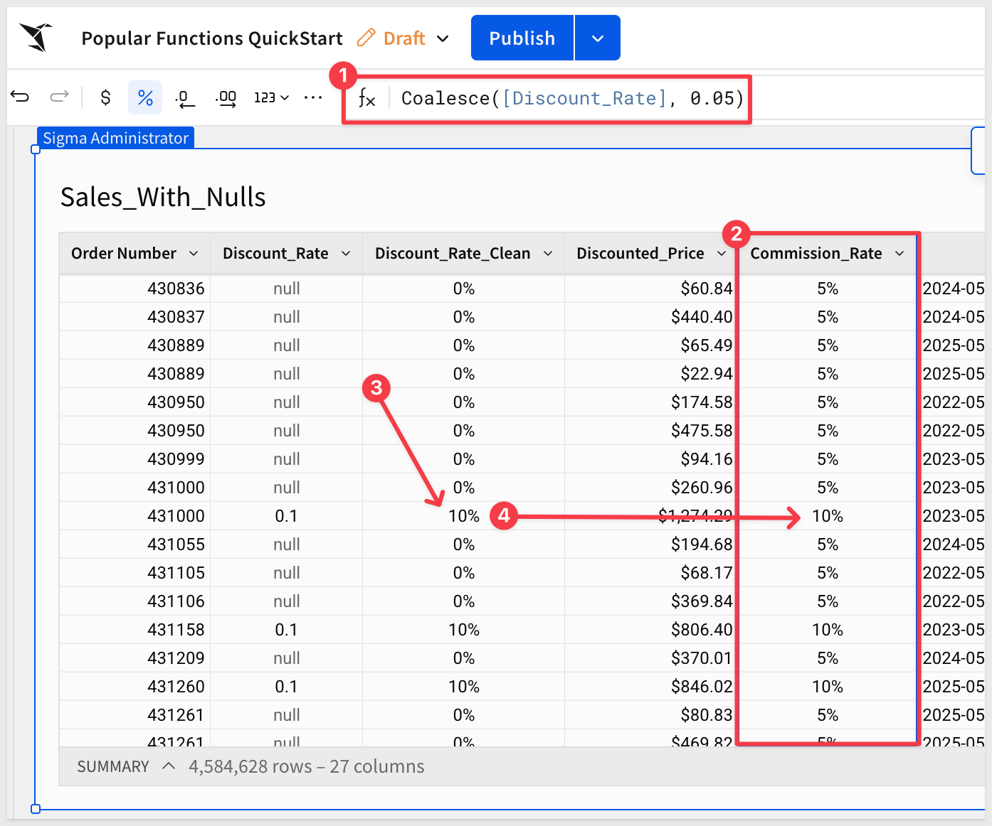
Coalesce()
Coalesce returns the first non-null value from a list of arguments. This is useful when you have multiple potential sources for a value.
For example, let's create a commission structure with fallback values. Add a new column:
Column Name:     Formula:
Commission_Rate  Coalesce([Discount_Rate], 0.05)
This will:
- Use the discount rate if it exists
- Otherwise default to 5% commission
You can also use Coalesce with multiple fallback values. For example:
Coalesce([PrimaryRate], [SecondaryRate], [DefaultRate], 0)
Click Publish.
For more information, see Zn and Coalesce
The Contains function checks if a text string contains a specific substring. This is useful for filtering, categorizing, or flagging records based on partial text matches.
Use case: Identify and categorize products by type (cables, chargers, adapters) to analyze sales by product category.
Create a new page and rename it to Contains.
Add a child table from the Data page's PLUGS_ELECTRONICS_HANDS_ON_LAB_DATA table.
Rename the table to Product_Categories.
Let's create columns that identify different product types. Add a new column:
Column Name:     Formula:
Is_Cable         Contains([Product Name], "Cable")
This returns True if the product name contains "Cable", otherwise False.
Now add a few more category columns:
Column Name:     Formula:
Is_Charger       Contains([Product Name], "Charger")
Is_Adapter       Contains([Product Name], "Adapter")
Is_USB           Contains([Product Name], "USB")
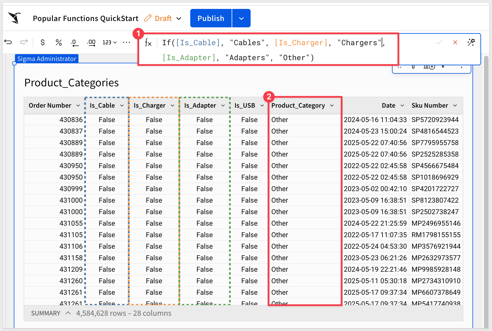
Now we can create a more readable product category column using these flags. Add a new column:
Column Name:      Formula:
Product_Category  If([Is_Cable], "Cables", [Is_Charger], "Chargers", [Is_Adapter], "Adapters", "Other")
With over 4 million rows, it can be hard to see the distribution. To do that quickly, we can look at column details:
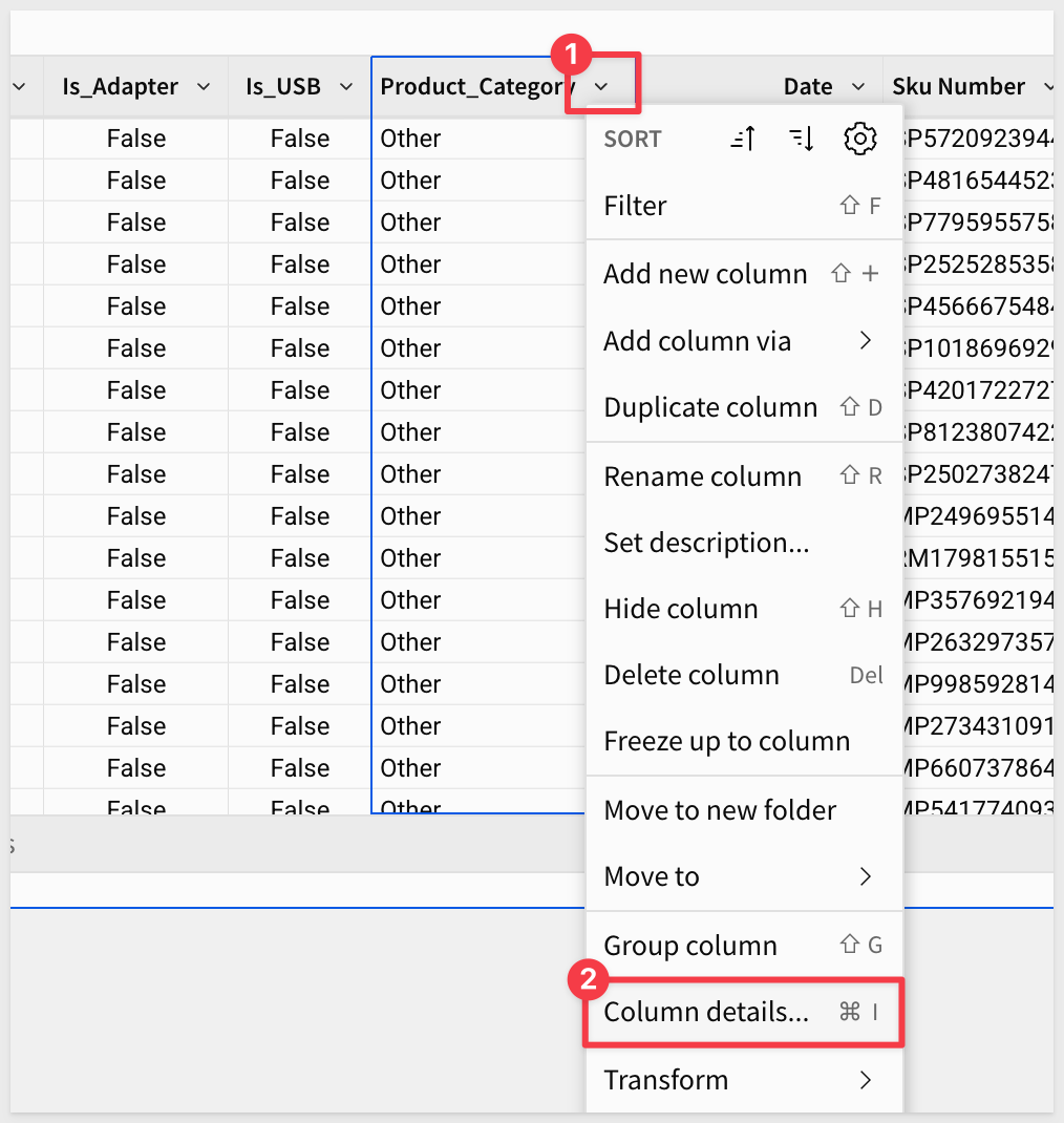
This shows lots of useful information about the selected column, including the distribution of values:
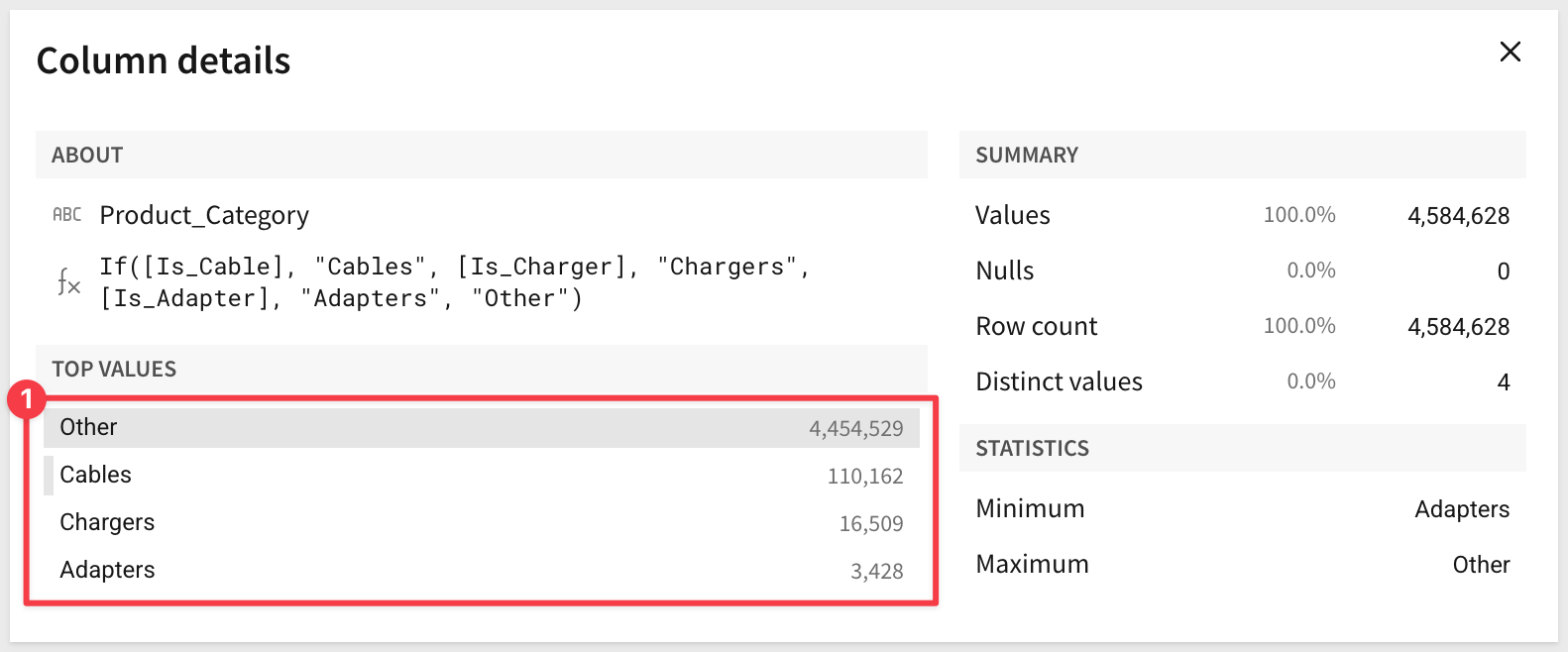
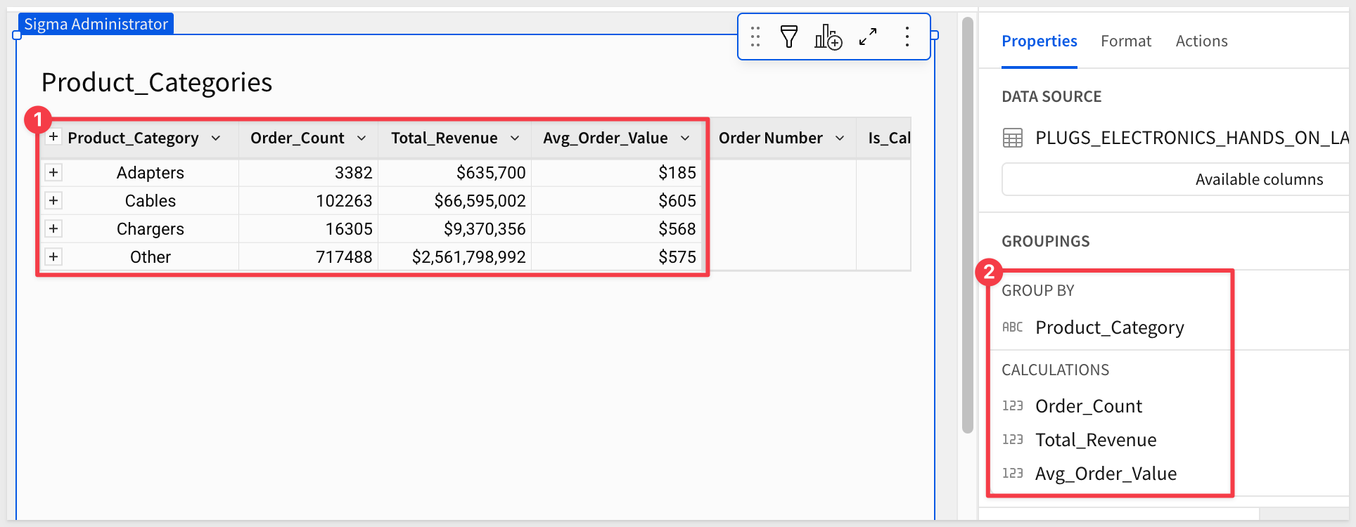
To make that visible in the table, we can group by Product_Category and add calculations to see sales by category.
Drag the Product_Category column to the GROUPINGS section.
Add a new calculation column:
Column Name:     Formula:
Order_Count      CountDistinct([Order Number])
You can also add other useful metrics:
Column Name:        Formula:
Total_Revenue       Sum([Order_Value])
Avg_Order_Value     Avg([Order_Value])
This analysis helps answer questions like:
- Which product categories generate the most revenue?
- What's the average order value by category?
- Which categories should we stock more inventory for?
Click Publish.
For more information, see Contains
The In function checks if a value matches any item in a list. This simplifies formulas that would otherwise require multiple OR conditions.
Use case: Analyze performance of specific high-value store regions to understand their contribution to overall sales.
Create a new page and rename it to In_Function.
Add a child table from the Data page's PLUGS_ELECTRONICS_HANDS_ON_LAB_DATA table.
Rename the table to Regional_Analysis.
Let's say leadership wants to focus on three key regions: West, South, and East. We can create a flag to identify orders from these regions.
Add a new column:
Column Name:      Formula:
Is_Key_Region     In([Store Region], "West", "South", "East")
This returns True for orders from these three regions, False for all others.
Without the In function, you would need to write:
[Store Region] = "West" Or [Store Region] = "South" Or [Store Region] = "East"
The In function is much cleaner and easier to maintain.
Now let's create a more readable column using this flag:
Column Name: Formula:
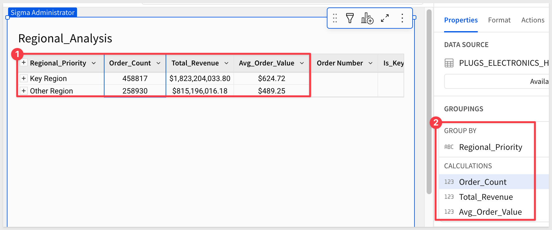
Regional_Priority If([Is_Key_Region], "Key Region", "Other Region")
Group by Regional_Priority and add calculations to compare performance:
Column Name:        Formula:
Order_Count         CountDistinct([Order Number])
Total_Revenue       Sum([Order_Value])
Avg_Order_Value     Avg([Order_Value])
This helps answer questions like:
- What percentage of revenue comes from key regions?
- Do key regions have higher average order values?
- Should we allocate more resources to key regions?
For more information, see In
Click Publish.
The IsNull and IsNotNull functions check whether a value is null or not. These are essential for data quality checks, conditional logic, and identifying incomplete records.
Use case: Identify data quality issues by flagging records with missing or incomplete information to ensure data integrity.
Create a new page and rename it to Null_Checks.
Add a child table from the Data page's PLUGS_ELECTRONICS_HANDS_ON_LAB_DATA table.
Rename the table to Data_Quality_Check.
Let's create a simulated scenario where some discount values might be missing. Add a new column:
Column Name:       Formula:
Sample_Discount    If([Order_Value] > 1000, 0.15, If([Order_Value] > 500, 0.10, null))
This creates discounts only for orders over $500, leaving smaller orders with null values.
Now let's use IsNull to identify records without discounts:
Column Name:         Formula:
Missing_Discount     IsNull([Sample_Discount])
This returns True for records where the discount is null.
We can also use IsNotNull to identify complete records:
Column Name:         Formula:
Has_Discount         IsNotNull([Sample_Discount])
These functions are commonly used in conditional logic. For example, create a status column:
Column Name:        Formula:
Discount_Status     If(IsNull([Sample_Discount]), "No Discount", "Discounted")
Group by Discount_Status to see the distribution:
Column Name:        Formula:
Order_Count         CountDistinct([Order Number])
Total_Revenue       Sum([Order_Value])
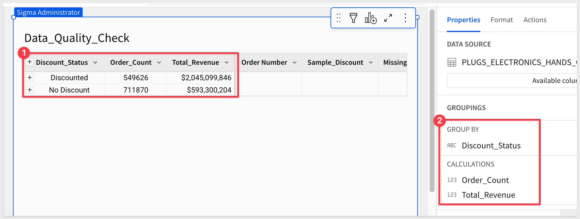
This helps answer questions like:
- What percentage of orders are missing discount information?
- How does revenue compare between discounted and non-discounted orders?
- Which records need follow-up for data completion?
For more information, see IsNull and IsNotNull
Click Publish.
Lookups allow you to enrich data in one table by pulling in columns from another table based on matching values (join keys).
Use case: Compare this year's sales performance against last year's sales by store region using lookup columns.
Lookups work by matching rows based on shared values between two columns—one from each table. Let's see how this works.
Create a new page and rename it to Lookups.
Add a child table from the Data page.
Rename the table to Regional_Sales_Performance.
Group by Store Region.
Now we'll create two additional tables to summarize sales by year. Add another child table from the Data page.
Rename this child table Sales_This_Year.
Group by Store Region.
Add another child table from the Data page and rename it Sales_Last_Year.
Group by Store Region as well.
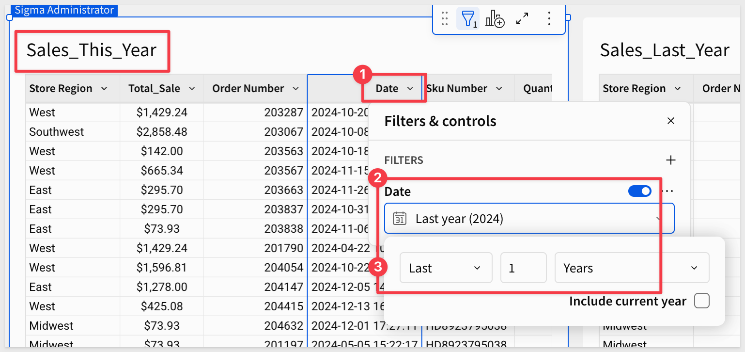
On the Sales_This_Year table, add a new column:
Column Name:     Formula:
Total_Sale       [Order_Value]
Add a filter on the Date column to show only this year's data.
On the Sales_Last_Year table, add the same Total_Sale column and filter to show only last year's data.
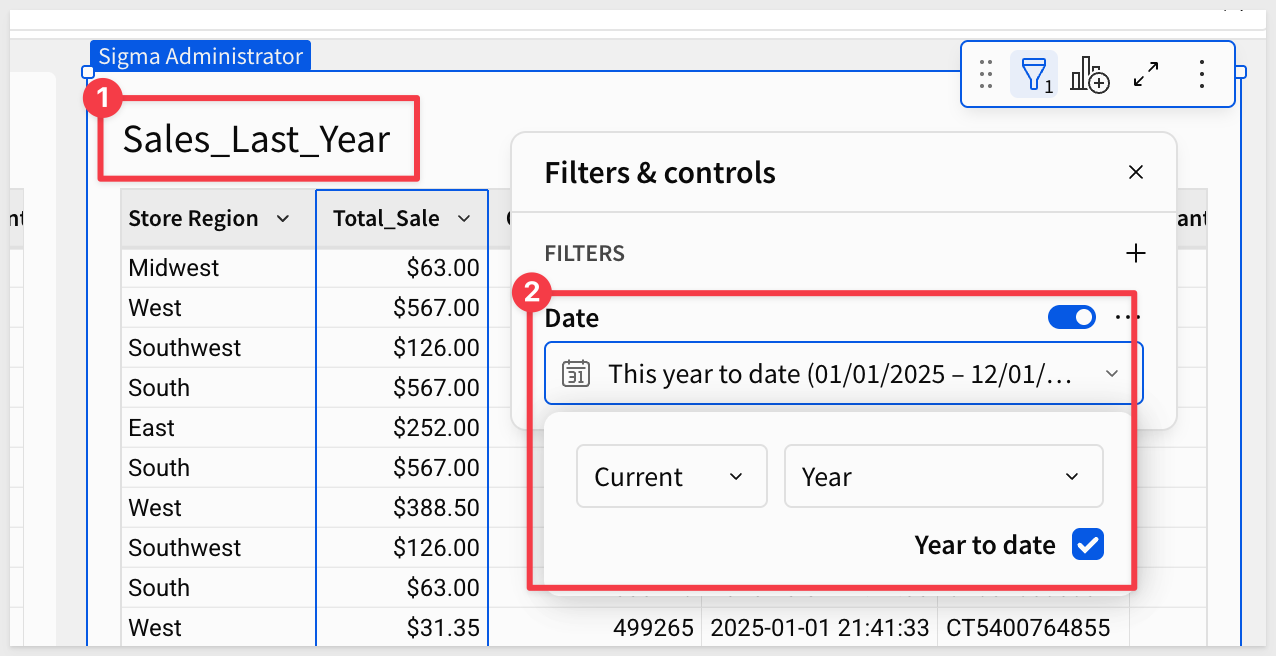
We have the two tables:
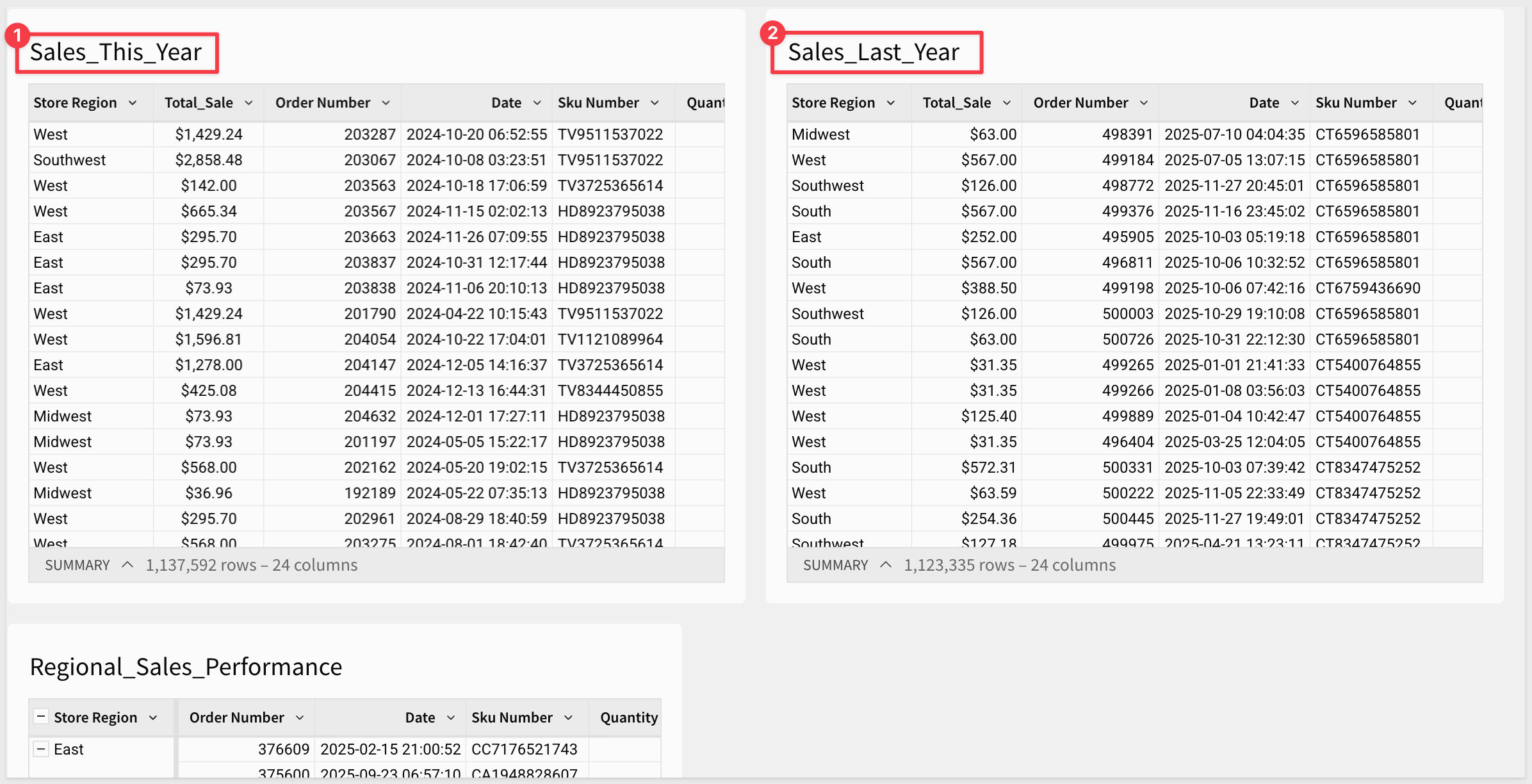
Now let's use lookups to bring both years' sales into the Regional_Sales_Performance table.
On the Regional_Sales_Performance table, open the menu for Store Region and select New column via lookup.
Configure the lookup:
- Select element: Choose
Sales_This_Year - Column to add: Select
Total_Sale - Aggregate: Select
Sum(this sums all sales for each region) - Map two elements: Match
Store Regionfrom both tables
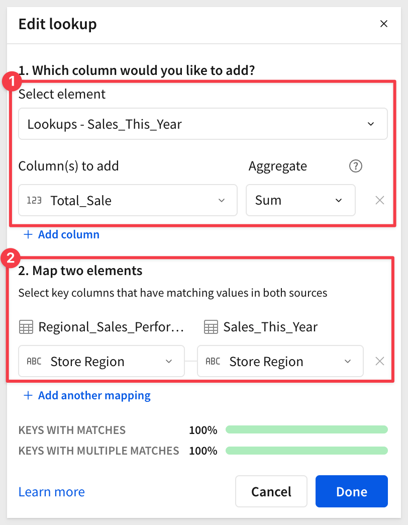
Click Done.
Rename the lookup column to This_Year_Sales and drag it to the CALCULATIONS section.
Repeat the process to add a lookup from Sales_Last_Year, rename it to Last_Year_Sales, and drag it to CALCULATIONS.
Now add a new column to see the year-over-year change:
Column Name:     Formula:
YoY_Change       ([This_Year_Sales] - [Last_Year_Sales]) / [Last_Year_Sales]
Format as percentage.
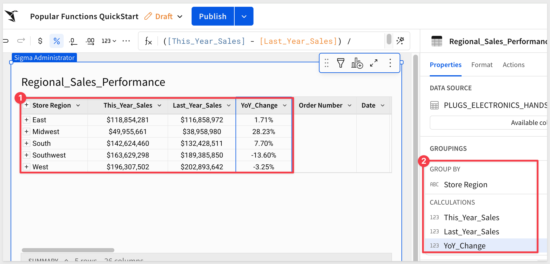
You now have a comparison table showing this year vs last year sales by region, with growth rates—all powered by lookups.
For more information, see Add columns through Lookup
Click Publish.
The PercentOfTotal function calculates what percentage each value represents of the total. This is essential for understanding relative contribution and distribution.
Use case: Analyze which stores contribute the most to their region's revenue to identify top performers and underperformers.
Create a new page and rename it to PercentOfTotal.
Add a child table from the Data page.
Rename the table to Store_Performance.
Group by Store Region, then add a nested grouping by Store Name.
Add a calculation for total sales by store:
Column Name:        Formula:
Store_Sales         Sum([Order_Value])
Format as currency.
Now add another calculation using PercentOfTotal:
Column Name: Formula:
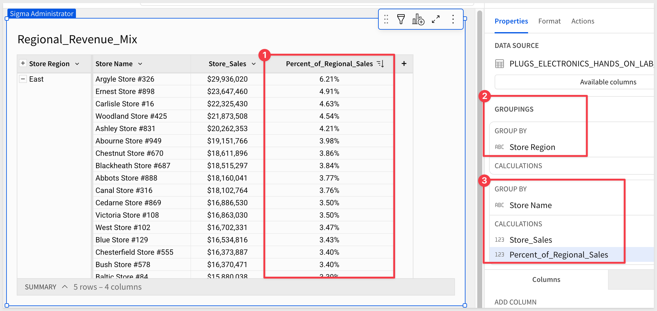
Percent_of_Regional_Sales PercentOfTotal(Sum([Store_Sales]))
Format as percentage.
The PercentOfTotal function automatically calculates each store's percentage within its region. Because of the grouping hierarchy, it calculates percentages at the Store Name level relative to the Store Region total.
Filter to show just one region to see the distribution more clearly. For example, filter to Store Region = "West":
Sort by Percent_of_Regional_Sales descending to see the ranking:
This helps answer questions like:
- Which stores are the top performers in each region?
- Are sales concentrated in a few stores or evenly distributed?
- Which underperforming stores need additional support?
You can remove the filter to see all regions and compare store performance across the entire company.
For more information, see PercentOfTotal
Click Publish.
The RegexpExtract function uses regular expressions (regex) to extract specific patterns from text strings. This is powerful for parsing structured data from unstructured text.
Use case: Extract product information from SKU numbers that follow a pattern to analyze sales by product type and model.
Create a new page and rename it to RegexpExtract.
Add a child table from the Data page's PLUGS_ELECTRONICS_HANDS_ON_LAB_DATA table.
Rename the table to SKU_Analysis.
Looking at the Sku Number column, we can see patterns like "SP5720923942", "MP2496955145", "CT6607378640", etc.
Let's say the pattern is: First 2 letters = Product Type, Next 4 digits = Model Number, Remaining digits = Serial Number.
Extract the product type (first 2 characters):
Column Name:     Formula:
Product_Type     RegexpExtract([Sku Number], "^([A-Z]{2})")
The pattern ^([A-Z]{2}) means:
^= Start of string([A-Z]{2})= Capture exactly 2 uppercase letters- Parentheses capture the match for extraction
Extract the model number (characters 3-6):
Column Name:     Formula:
Model_Number     RegexpExtract([Sku Number], "^[A-Z]{2}([0-9]{4})")
The pattern ^[A-Z]{2}([0-9]{4}) means:
- Skip first 2 letters (not captured)
([0-9]{4})= Capture exactly 4 digits
Extract the serial number (remaining digits):
Column Name:       Formula:
Serial_Number      RegexpExtract([Sku Number], "([0-9]{6,})$")
The pattern ([0-9]{6,})$ means:
([0-9]{6,})= Capture 6 or more digits$= End of string
Now group by Product_Type to analyze sales by product category:
Column Name:        Formula:
Order_Count         CountDistinct([Order Number])
Total_Revenue       Sum([Order_Value])
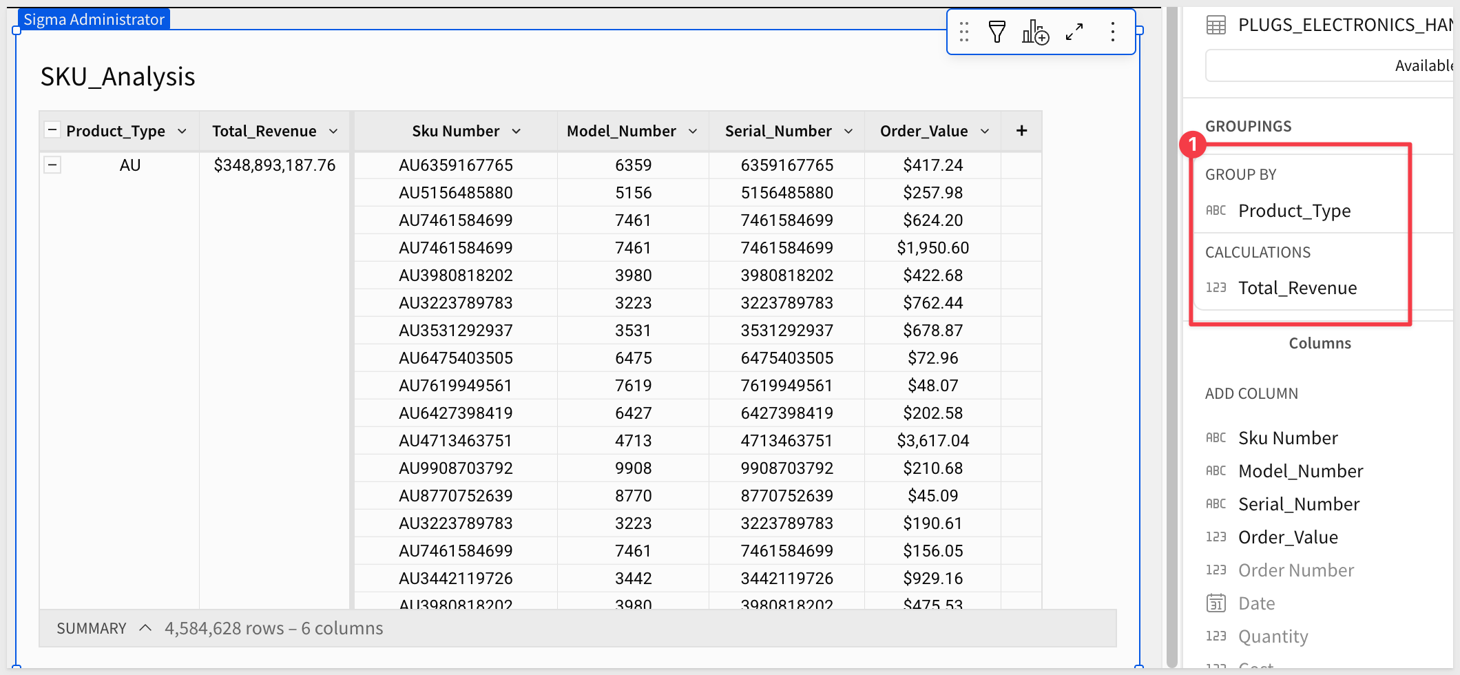
This helps answer questions like:
- Which product types (SP, MP, CT, etc.) are most popular?
- What's the revenue distribution by product type?
- Are certain model numbers performing better than others?
For more information, see RegexpExtract
Click Publish.
The Subtotal() function calculates aggregations at different levels within your data hierarchy. It's particularly useful for creating subtotals in pivot tables and calculating values at specific grouping levels.
Use Case: Analyze regional sales performance by calculating both store-level sales and regional subtotals to understand each store's contribution to its region's total.
Create Analysis Page
Create a new page and rename it to Subtotal.
Add a child table from the Data page's PLUGS_ELECTRONICS_HANDS_ON_LAB_DATA table.
Rename the table to Regional_Analysis.
Add Regional Grouping
In the Regional_Analysis table, click the Grouping icon and add two levels:
Store Region
Store Name
This creates a hierarchical view showing stores grouped by their region.
Calculate Store Sales
Click the + icon in the table header to add a new column:
Column Name:     Formula:
Store_Sales      Sum([Order_Value])
This shows total sales for each store.
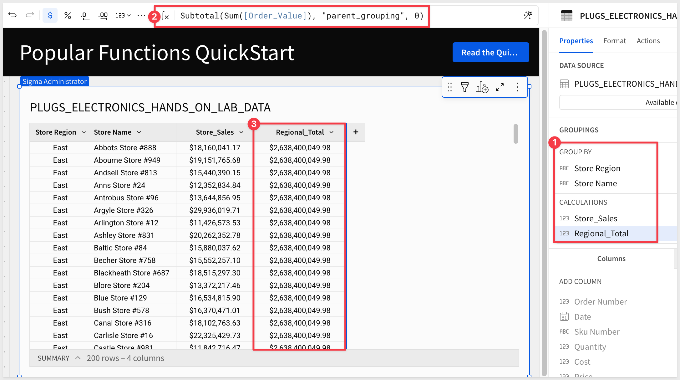
Add Regional Subtotal
Click the + icon to add another calculated column:
Column Name:       Formula:
Regional_Total     Subtotal(Sum([Order_Value]), "parent_grouping", 0)
The Subtotal() function with "parent_grouping" mode and parameter 0 calculates the total at the immediate parent grouping level. This displays the regional total on each store row, making it easy to compare individual store performance against the regional total.
Notice that each store in the East region shows the same Regional_Total value (for example, $2,638,400,049.98). This is expected behavior - it's showing the total for all East region stores combined. Each store row displays its own Store_Sales alongside the complete regional total, enabling easy comparison.
Calculate Store Contribution
Click the + icon in the groups calculations to add one more column:
Column Name:           Formula:
Percent_of_Region      [Store_Sales] / [Regional_Total]
Format this column as Percentage to show what portion of regional sales each store represents.
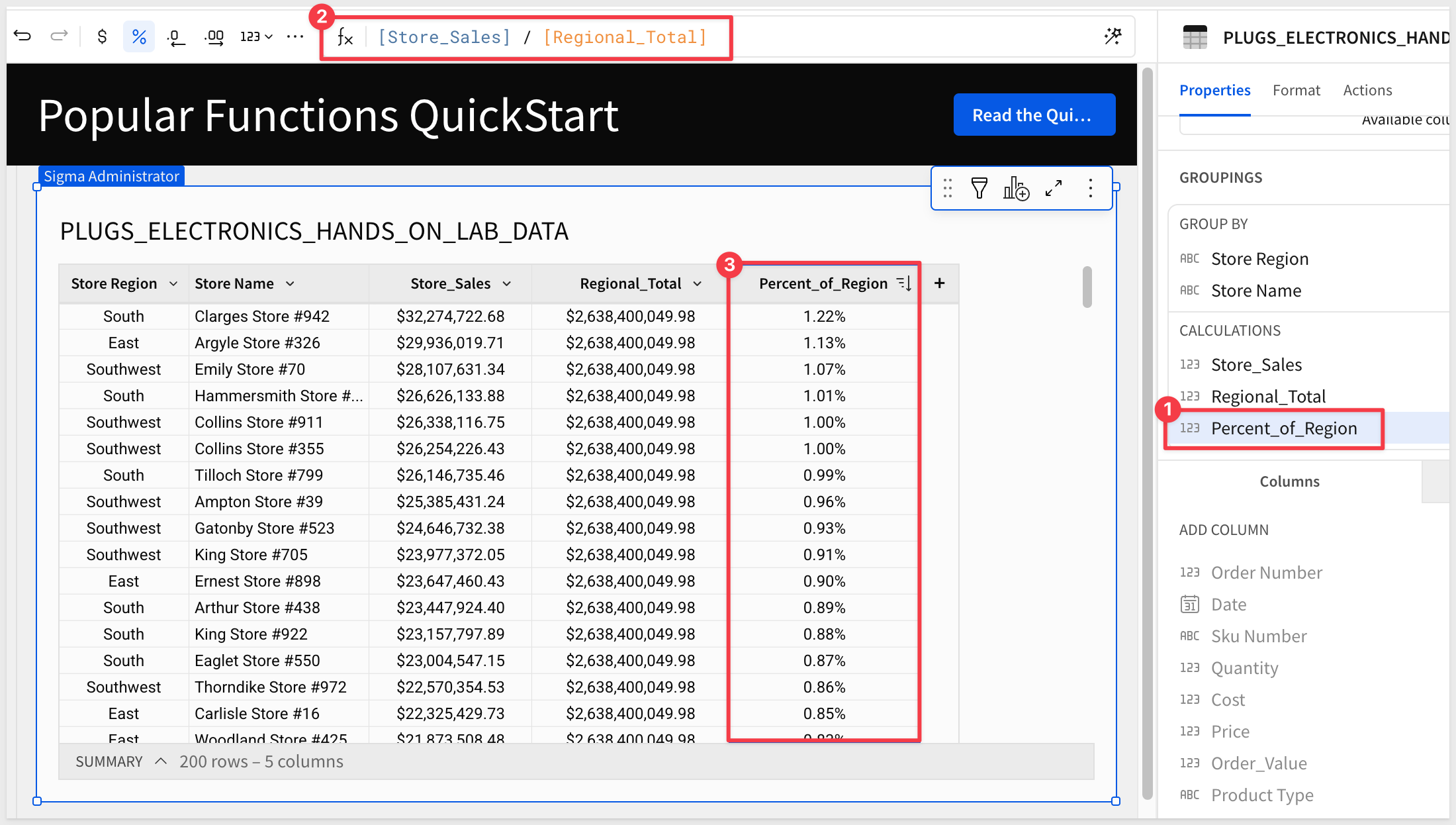
Business Insight: This analysis reveals which stores are the strongest performers within their regions. For example, you might discover that certain stores contribute much less of their region's total sales, indicating low-performing locations worth investigating.
This helps answer questions like:
- Which stores are the top performers in each region?
- Are regional sales concentrated in a few stores or evenly distributed?
- Which regions have the most balanced store performance?
For more information on the Subtotal function, click here.
Click Publish.
The Switch() function evaluates multiple conditions and returns different values based on which condition is true. It's a cleaner alternative to nested If statements when you have multiple scenarios to handle.
Use Case: Categorize stores into performance tiers based on their sales volume to identify high, medium, and low performers for targeted management strategies.
Create Analysis Page
Create a new page and rename it to Switch.
Add a child table from the Data page's PLUGS_ELECTRONICS_HANDS_ON_LAB_DATA table.
Rename the table to Store_Performance.
Group by Store
In the Store_Performance table, click the Grouping icon and add:
Store Name
This groups all orders by store.
Calculate Store Revenue
Click the + icon in the table header to add a new column:
Column Name:       Formula:
Store_Revenue      Sum([Order_Value])
This calculates total revenue for each store.
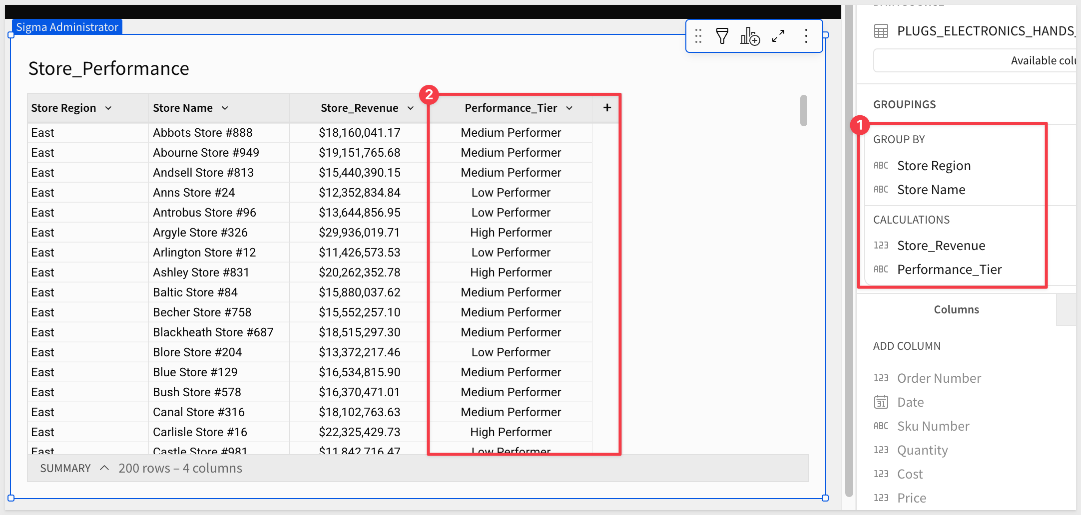
Add Performance Tier
Click the + icon to add another calculated column:
Column Name:         Formula:
Performance_Tier     Switch(True, [Store_Revenue] >= 20000000, "High Performer", [Store_Revenue] >= 15000000, "Medium Performer", [Store_Revenue] >= 10000000, "Low Performer", "Underperforming")
The Switch() function starts with True as the first parameter, then evaluates condition-result pairs in order, returning the first matching result:
- Stores with $20M+ revenue are "High Performers"
- Stores with $15M-$20M are "Medium Performers"
- Stores with $10M-$15M are "Low Performers"
- All others (less than $10M) are "Underperforming"
The final value "Underperforming" acts as a default, catching any stores that don't meet the previous criteria.
Visualize Performance Distribution
To better see the distribution of stores across performance tiers, add a bar chart.
Add a Child > Chart from the Store_Performance table.
Configure the chart:
- X-Axis: Performance_Tier
- Y-Axis: Store_Revenue (Aggregation: Sum)
Now we can easily see the underperforming stores; right-click and Drill down to explore the underlying data:
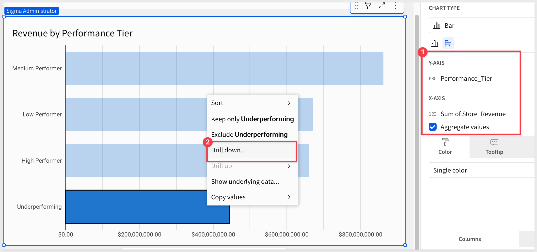
Drill by Store_Name and tap the spacebar to see a chart and table data:
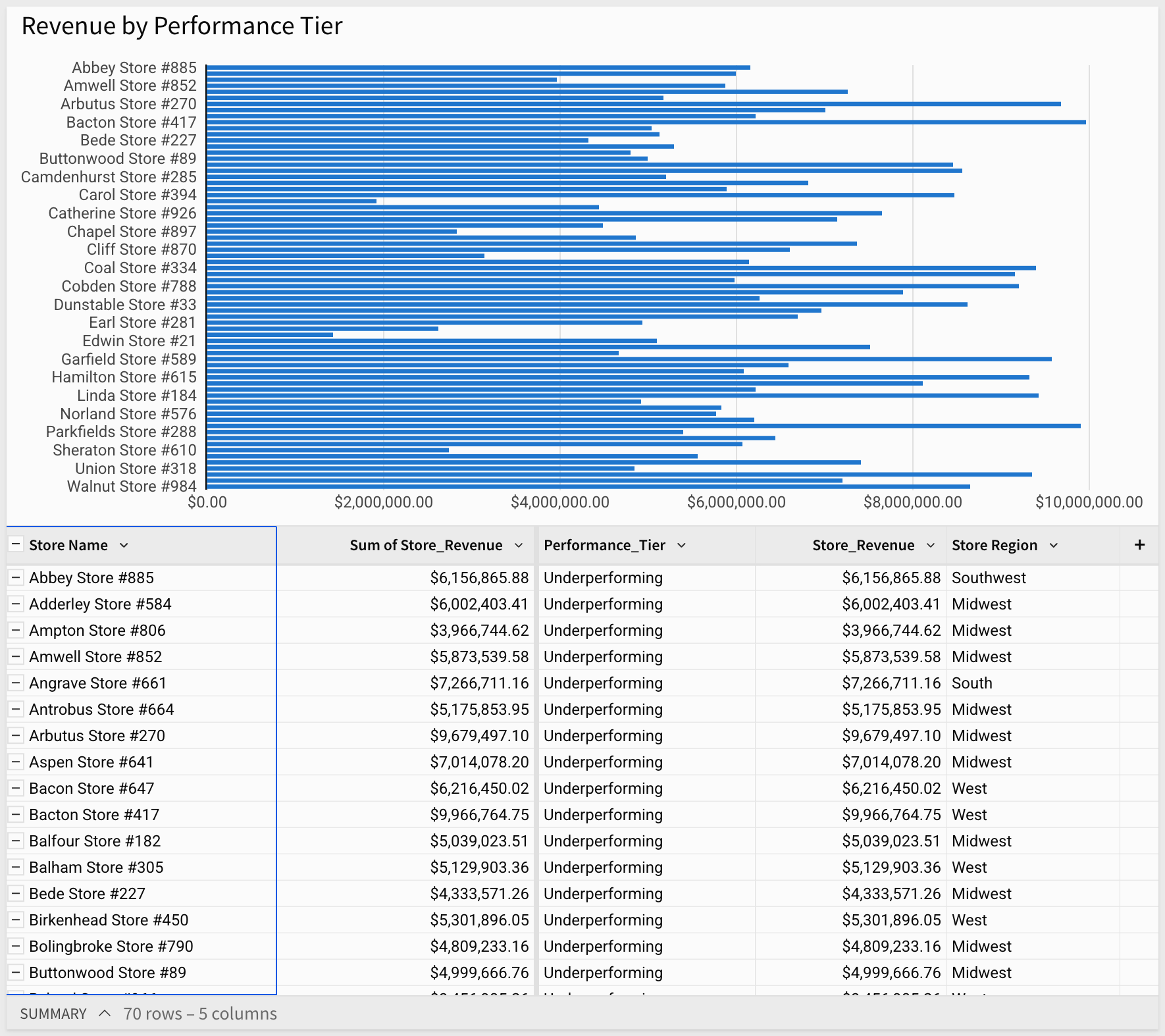
Business Insight: The bar chart reveals your store portfolio's performance distribution at a glance. You can quickly see the total revenue contribution from each tier and identify how many stores fall into each category. This segmentation enables targeted strategies - high performers can be studied for best practices, medium performers can be pushed toward high performance, and underperformers require intervention or evaluation.
For more information on the Switch function, click here.
Click Publish.
In this QuickStart, we explored some of Sigma's most frequently used functions through practical business scenarios.
Sigma supports over 200 functions that enable you to perform simple and complex calculations, transformations, and extractions to get the most out of your data.
For the full listing see our Function index
Additional Resource Links
Blog
Community
Help Center
QuickStarts
Be sure to check out all the latest developments at Sigma's First Friday Feature page!