This QuickStart is part of a series designed to instruct new users how to use Sigma to explore and analyze data using Tables.

This QuickStart assumes you have already taken the QuickStart "Fundamentals 1: Getting Around" and are now familiar with Sigma's user interface (UI). Given this, some steps are assumed to be known and may not be shown in detail.

If you're familiar with traditional spreadsheet tools, such as Excel, you are likely to associate data and formulas with individual cells. While Sigma Tables are very spreadsheet-like, data is managed at the column level rather than on individual cells. This means actions such as calculations and formatting changes are applied to every cell in a column.

Managing data at the column level ensures consistency and accuracy, and prevents common errors, across large and ever-growing sets of data.

We will be working with some common sales data from our fictitious company ‘Plugs Electronics'. This data is provided to you automatically. We will look at sales data, but throughout the course of other QuickStarts will incorporate more sources from associated store, product, and customer data.

The other "Fundamental" QuickStarts explore topics such as working with Visualizations, Pivot Tables, Dashboards and more. We have broken these QuickStarts up so that they can be taken in any order you want, except the "Getting Around" QuickStart should be taken first.

Target Audience

Sigma combines the unlimited power of the cloud data warehouse and the familiar feel of a spreadsheet; no limit on the amount of data you wish to analyze. Sigma is awesome for users of Excel and even better for customers who have millions of rows of data.

Typical audience for this QuickStart are users of Excel, common business intelligence or reporting tools and semi-technical users who want to try out or learn Sigma. Everything is done in a browser so you already know how to use that. No SQL or technical skills are needed to do this QuickStart.

Prerequisites

• A computer with a current browser. It does not matter which browser you want to use.
• Completion of the QuickStart "Fundamentals 1: Getting Around"
• Access to your Sigma environment. A Sigma trial environment is acceptable and preferred.
• If have not already, you can sign up for a Sigma Trial here:

Free Trial

What You'll Learn

Through this QuickStart we will walk through how to access sample data to build a table, add new calculated columns, group and filter data and apply conditional formatting.

Our starting point is the "Plugs Sales" Workbook created in the "Fundamentals 1: Getting Around" QuickStart.

In Sigma, open the Workbook Plugs Sales and place it in edit mode. We should still have the Page tab called Data that has the "Plugs Sales" Table on it.

Our source data in Snowflake is missing a few columns that we want users to have access to, but we want to control how the column values are calculated.

The two missing column are Revenue and Profit.

Click the column dropdown from the Price column and select Add new column.

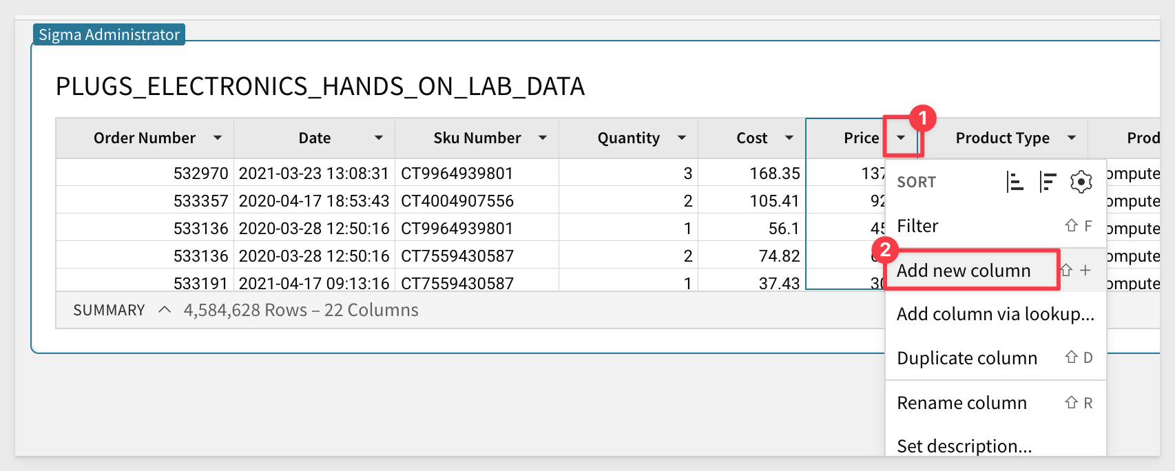
Rename the new column Revenue.

Enter the formula:

[Price] * [Quant] 

This is an intentional mistake in our formula; Quant is not a valid column and it does not exist anywhere else in the Workbook. What happened?

Sigma makes you immediately aware the function has a problem:

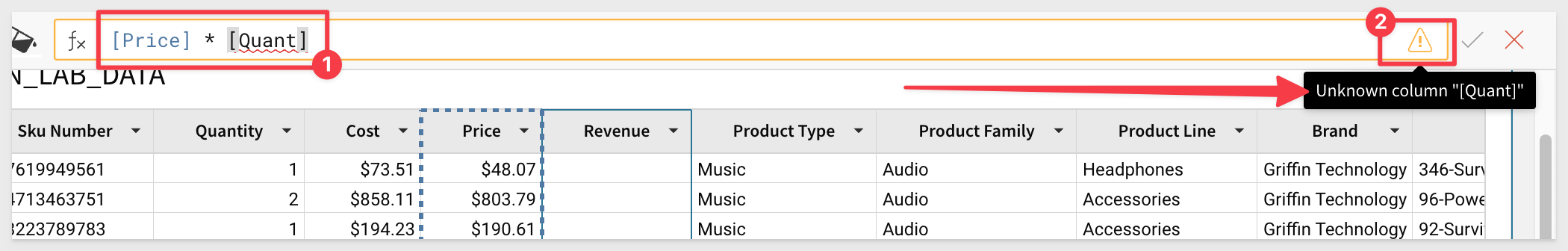
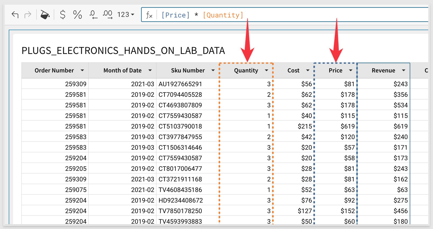
Easy to fix, just adjust the column name to Quantity and click the checkmark at the end of the Function bar. Simple!

Now that we have our Revenue, we should be able to calculate our Profit.

You can do this one yourself now:

[Revenue] - [Cost]

Lastly, click the Cost column, hold down shift on your keyboard and click the Profit column. All four columns are selected now.

Apply currency formatting to them all at once:

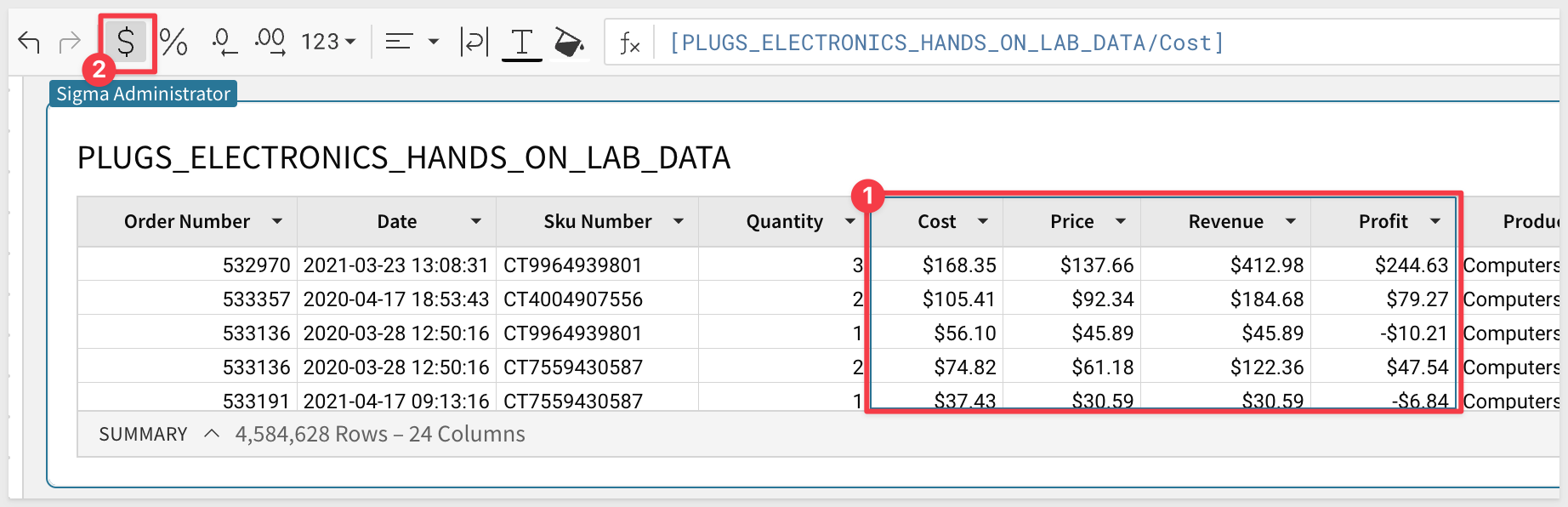
We now have source data that we can reuse as we go forward.

Add a new Page and name it Tables. Your Workbook should look like this:

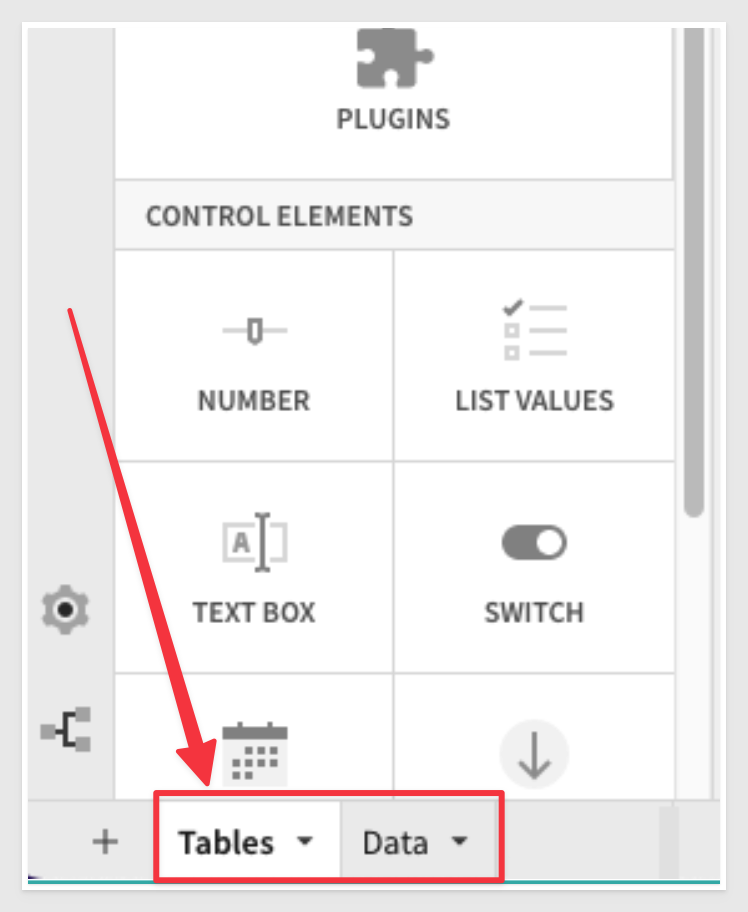
Click the + icon to open the Editor Panel. This panel gives you access to all the objects possible to add to a Page.

Select Table and for the source of data; we will use the table on the workbooks's Data page (under PAGE ELEMENTS):

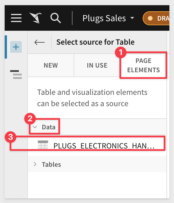
Notice that there are a few options for the source data. Reusing data that has already been queried from the Connection can help improve performance by limiting the number of queries sent to the Cloud Data Warehouse (CDW).

• New: Allows you to obtain data from any of your Connections.
• In Use: Allow you use source data that is already in use on another Page in this Workbook
• Page Elements: Table and visualization elements can be selected as a source from the open Workbook

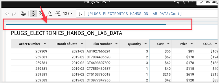
We now have our table and can begin working just like a normal spreadsheet. Get ready, you may be pleasantly surprised by how easy this is in Sigma.

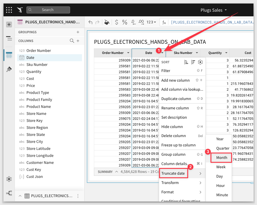
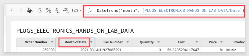
First, let's truncate the Date column to Month. You can do this by selecting the dropdown on the header column for Date and select Truncate date and click Month.

Sigma makes things easy for you but there is a ton of power being applied in the background to make it that way.

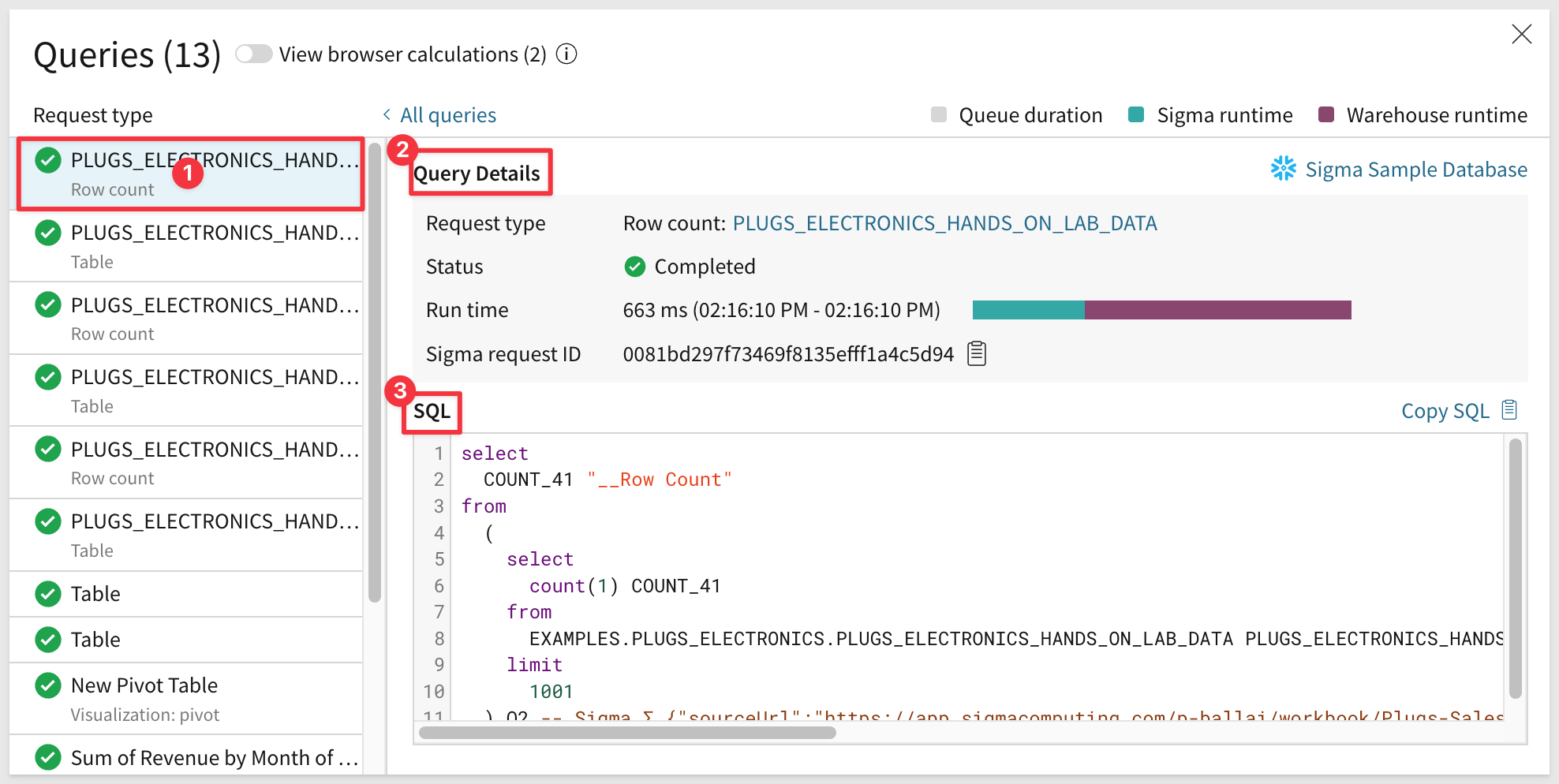
At any time you can click on the dropdown next to the refresh icon and select the query history to see exactly what is being run each time a change is made. This can be very useful for those with knowledge of SQL.

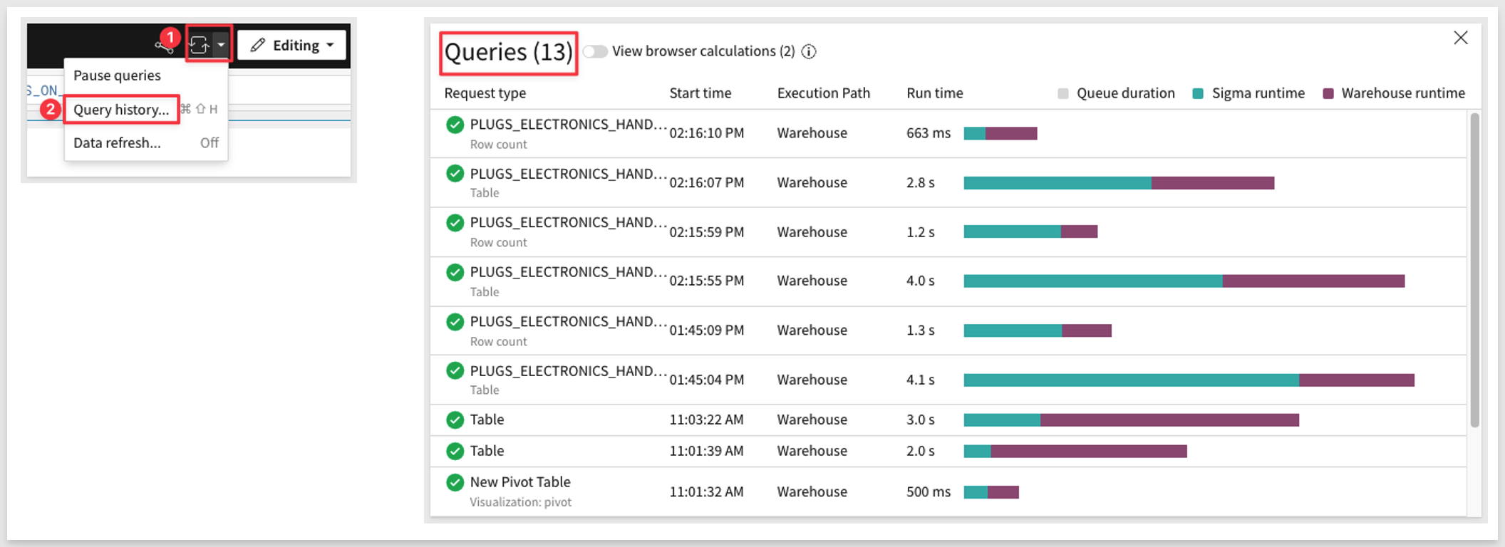
Clicking into the first Query gives every last detail:

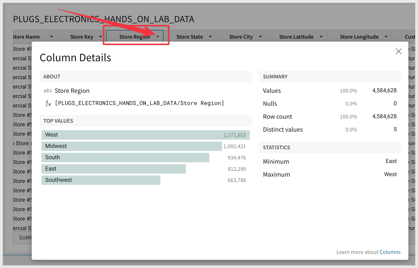
Related to the last item there is another feature that lets you "peek" behind a column to see some useful information. Click on the column Store Region's drop list and click Column Details. This will display a pop-up to help you see things like Top Values and if nulls exist and more:

There are times when a column has not been made available in the source data. It is still possible for users to add them (assuming they have been granted permission).

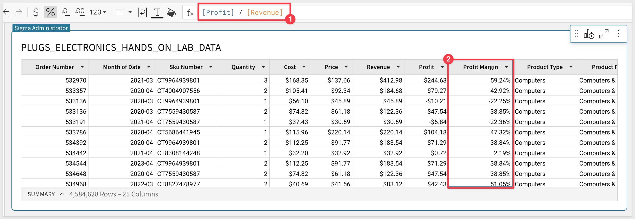
We know our profit made for each transaction, but we also are interested to know the Profit Margin percentage on each item. Add a new column (next to Profit), and use the formula:

[Profit] / [Revenue]

Rename the column Profit Margin In this case, change the formatting to a %.

Your Page should now look similar to this:

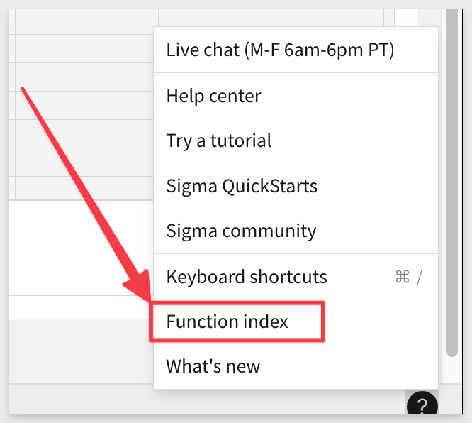
Some of these functions have been pretty easy, but Sigma is capable of performing the most commonly used functions available in excel/google sheets or SQL. We will get into some more advanced functions later, but you can always check out the complete list by clicking the ‘Help' button in the lower right hand corner and selecting Function Index

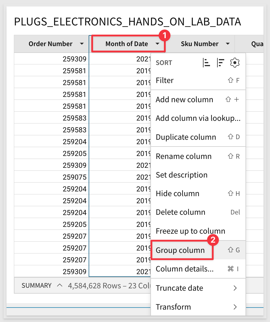
So far we have done some pretty simple operations. Let's go a bit deeper and group the data, building on the work we just did. There are two ways to group data. One is selecting the column and using the drop list and clicking "Group column".

This works fine but there is another method that introduces you to using the element configuration panel.

Using the Element Panel (and with the table selected) just drag and drop the Month of Date column up to the GROUPINGS section as shown below:

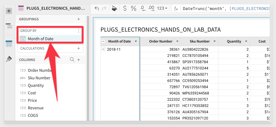
The table will automatically group on this column which allows us to perform calculations at his level of grouping.

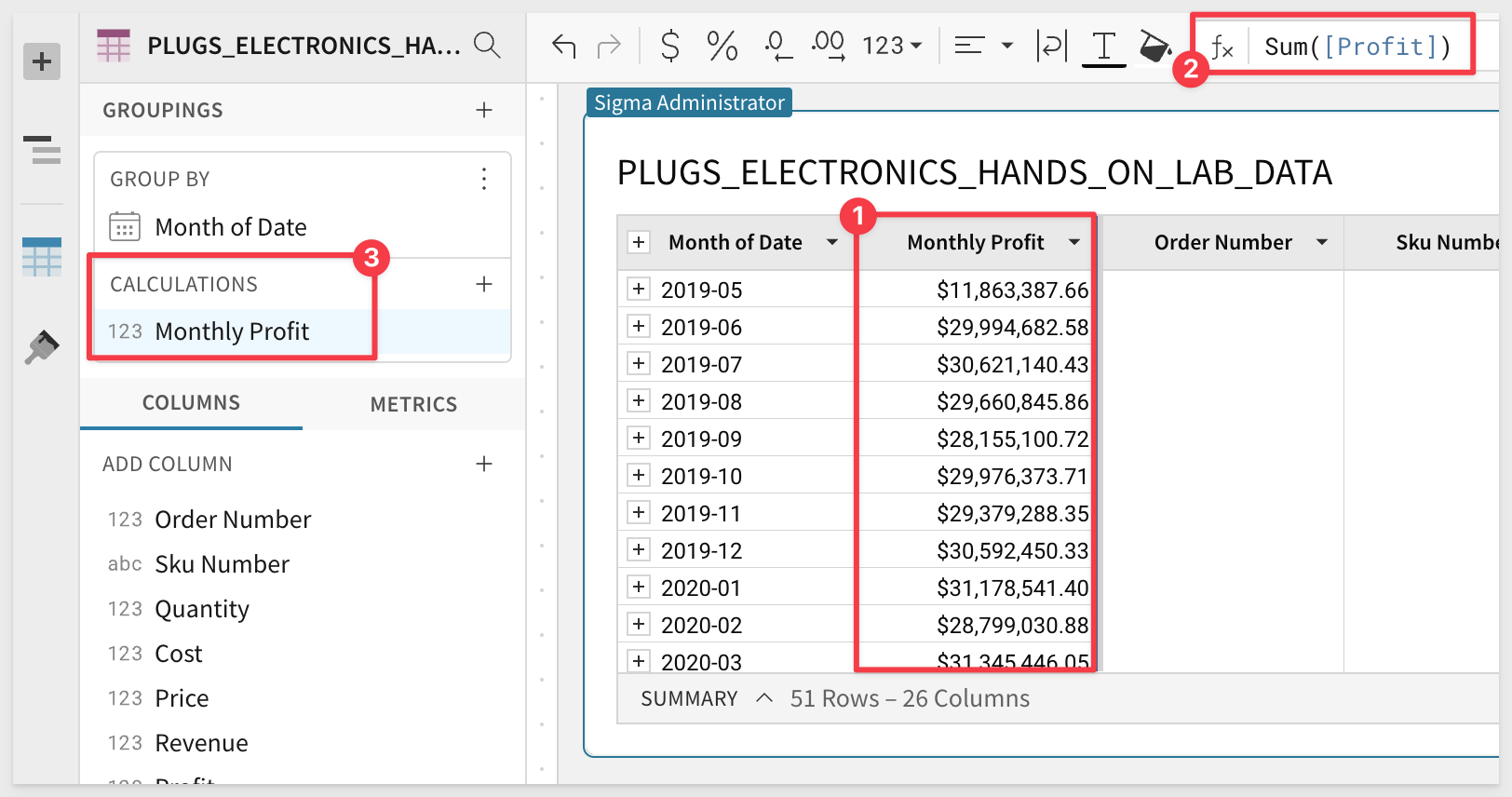
Using the Month of Date column's drop arrow, add a New column and rename it Monthly Profit:

Use the following formula:

Sum([Profit])

Notice how the new column is part of the Element panel / Grouping / Calculation under Month of Date?

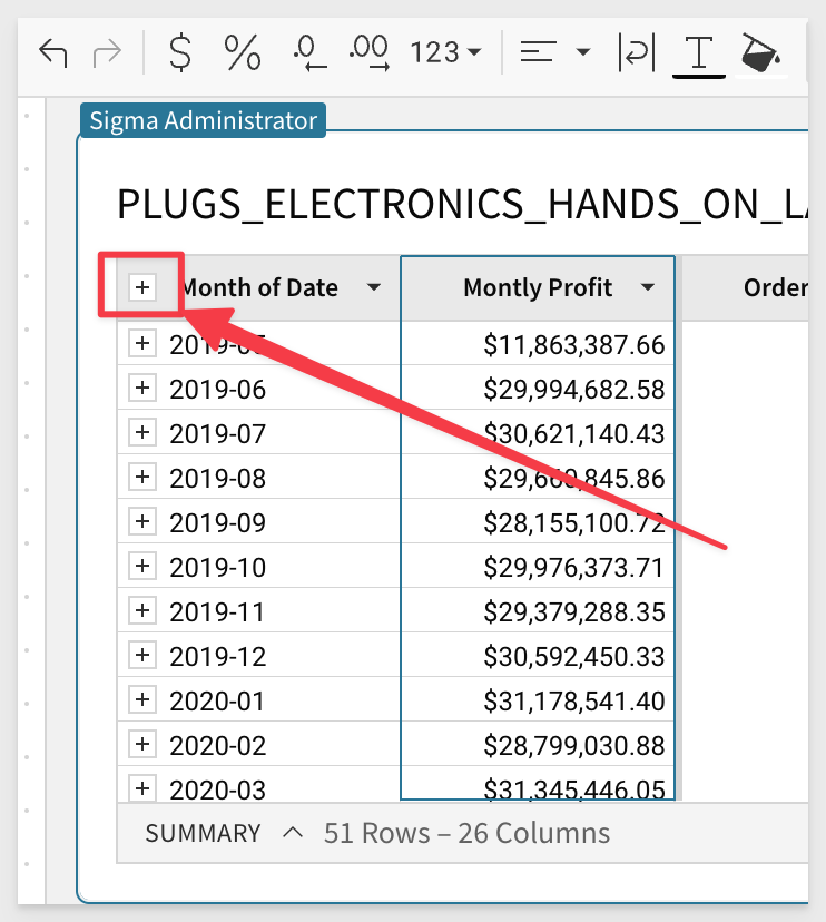
You can at any point collapse a single month, or all the months to hide the underlying data. You can do this by clicking the minimize hash next to the column header of Month of Date or any Monthly values.

Click on the minimize hash next to Month of Date to collapse all the Months.

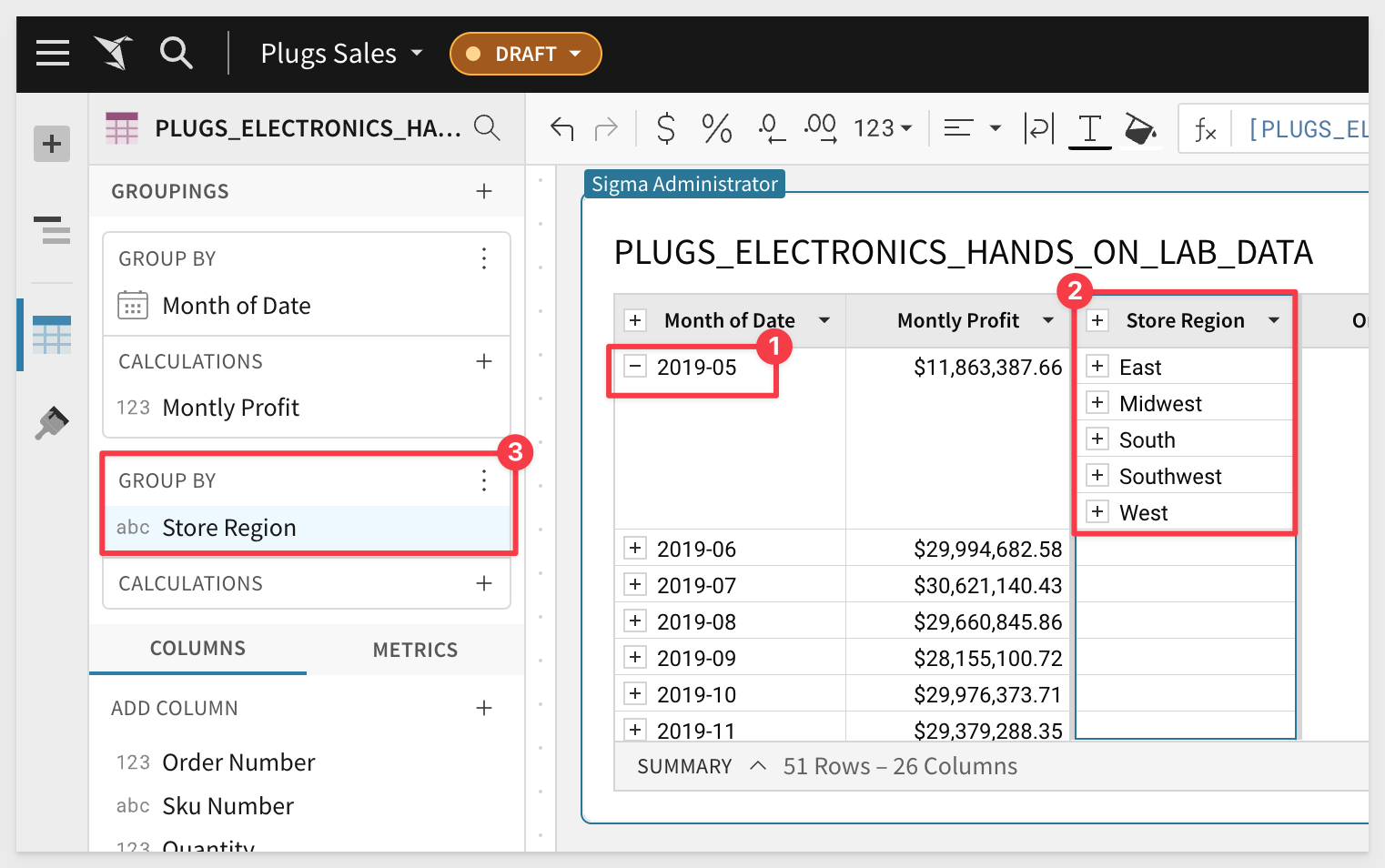
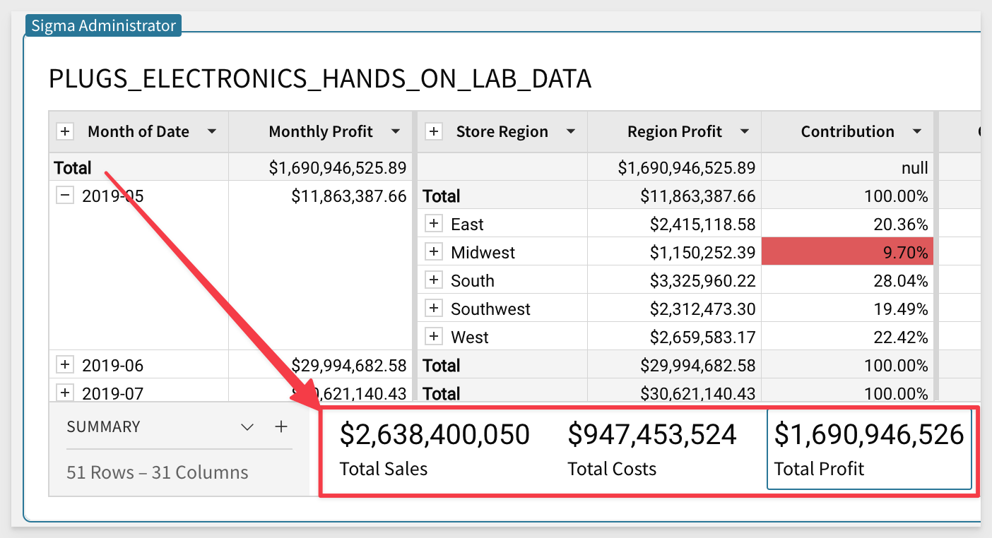
Scrolling to the right of the table, find the column Store Region. Using the dropdown, select Group column.

Scrolling back to the left, you see that we have created another grouping below the Month grouping. We can now perform calculations at this grouping level. You may want to expand just the first Month of Date to see the Store Region groups:

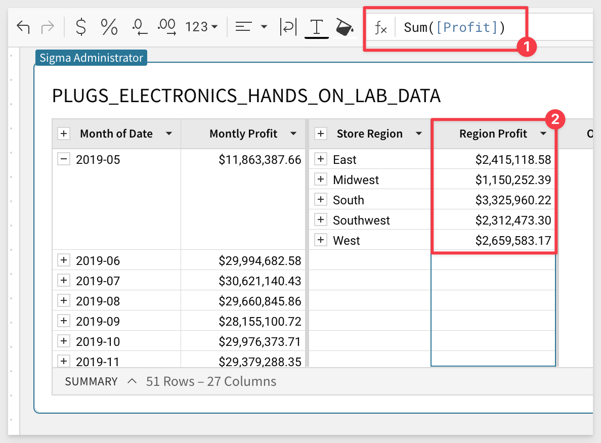
Let's add a new column next to Store Region for Region Profit using the formula:

Sum([Profit])

We can now see all our months and regional profits.

Taking this one step further, we can also perform calculations across the different grouping levels.

Clicking the dropdown next to Region Profit, select Add new column. Use the formula:

[Region Profit] / [Monthly Profit]

Format this as a percentage.

Rename the column Contribution:

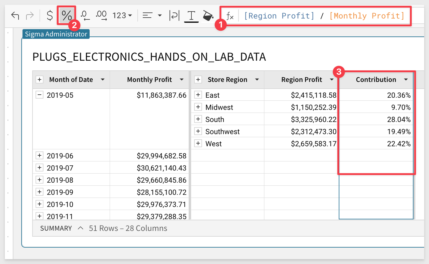
We can now see exactly how much each region is contributing to the monthly profit.

There are no limitations in Sigma tables for how many groupings you can have.

You can also swap the order of the groupings in the left hand pane using a simple drag and drop method. We will leave the groupings alone for now.

Sigma Workbook Tables have many ways to get totals, sub-totals, and summary values. We will explore them now.

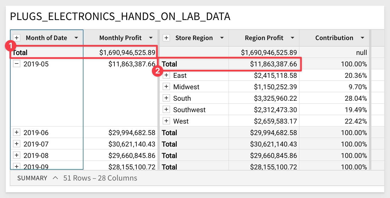
First, from the Store Region column header dropdown, select Show Totals.

You can now see we have totals aggregated at the Regional levels:

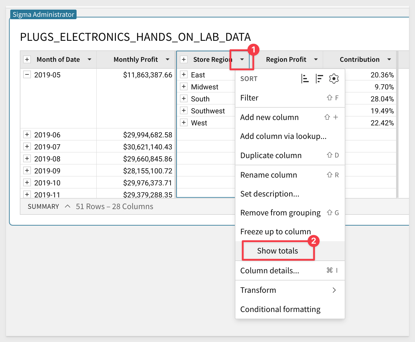
Taking this a step further we can do the same thing for our months. From the Month of Date column header dropdown, select Show Totals.

We now have totals at the Monthly level as well.

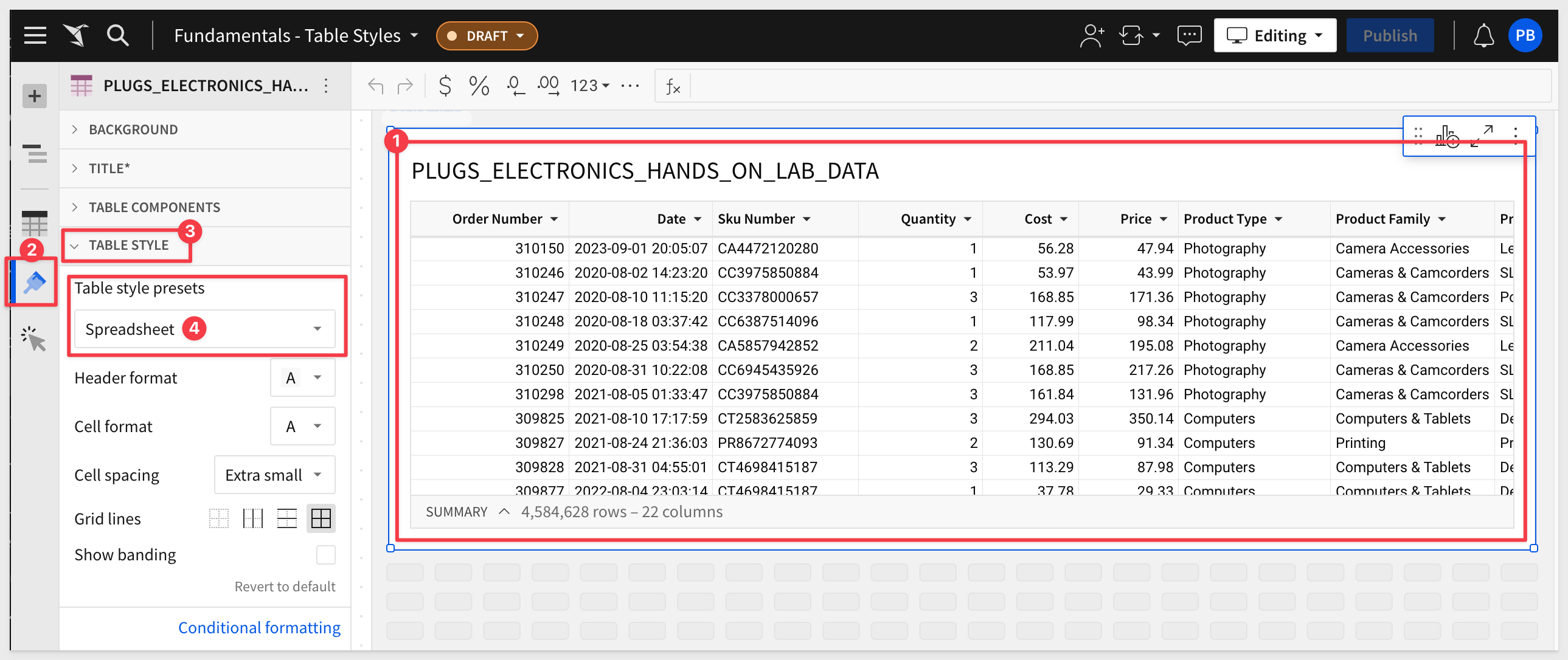
When working with tables, Sigma provides style presets for out-of-the-box aesthetics and readability. You can customize all style components independently for more personalized table designs.

There are two table presets that can be quickly set and then further customized to suit your needs.

Spreadsheet

This preset, which is the default for new tables, is designed for ongoing analysis and collaboration and will feel familiar to uses of Excel or Google Sheets.

For example, in this new table, we can see that the default Table Style is automatically set to Spreadsheet and there are additional customization options:

Presentation

Changing the setting Table Style to Presentation results in this:

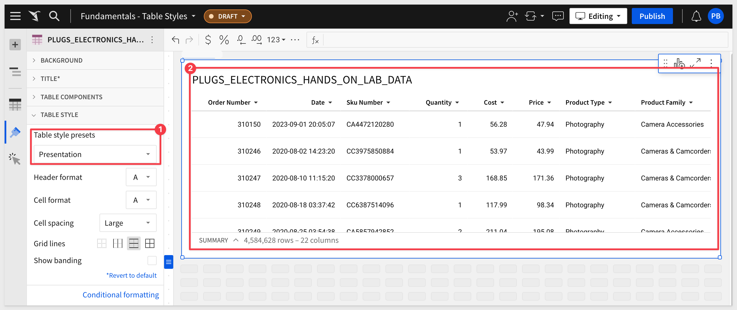
This preset is designed is ideal for aligning with company branding and adding visual appeal to your workbook:

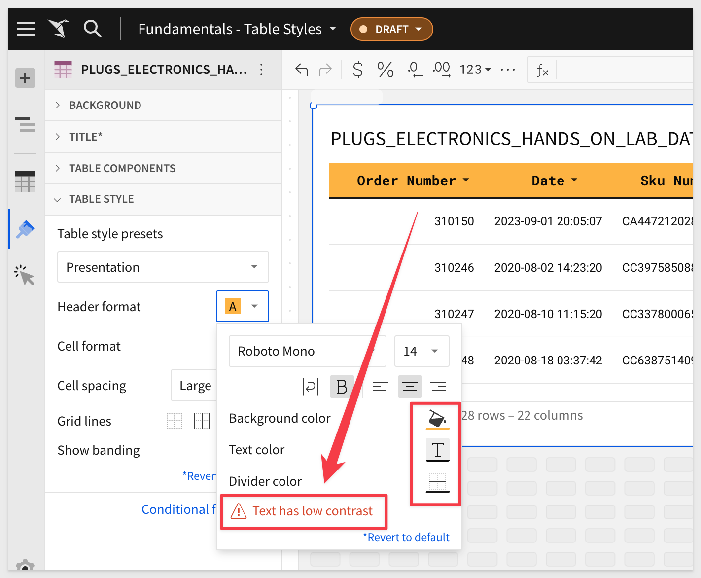
Sigma will warn you if the styling set is problematic for some people. For example:

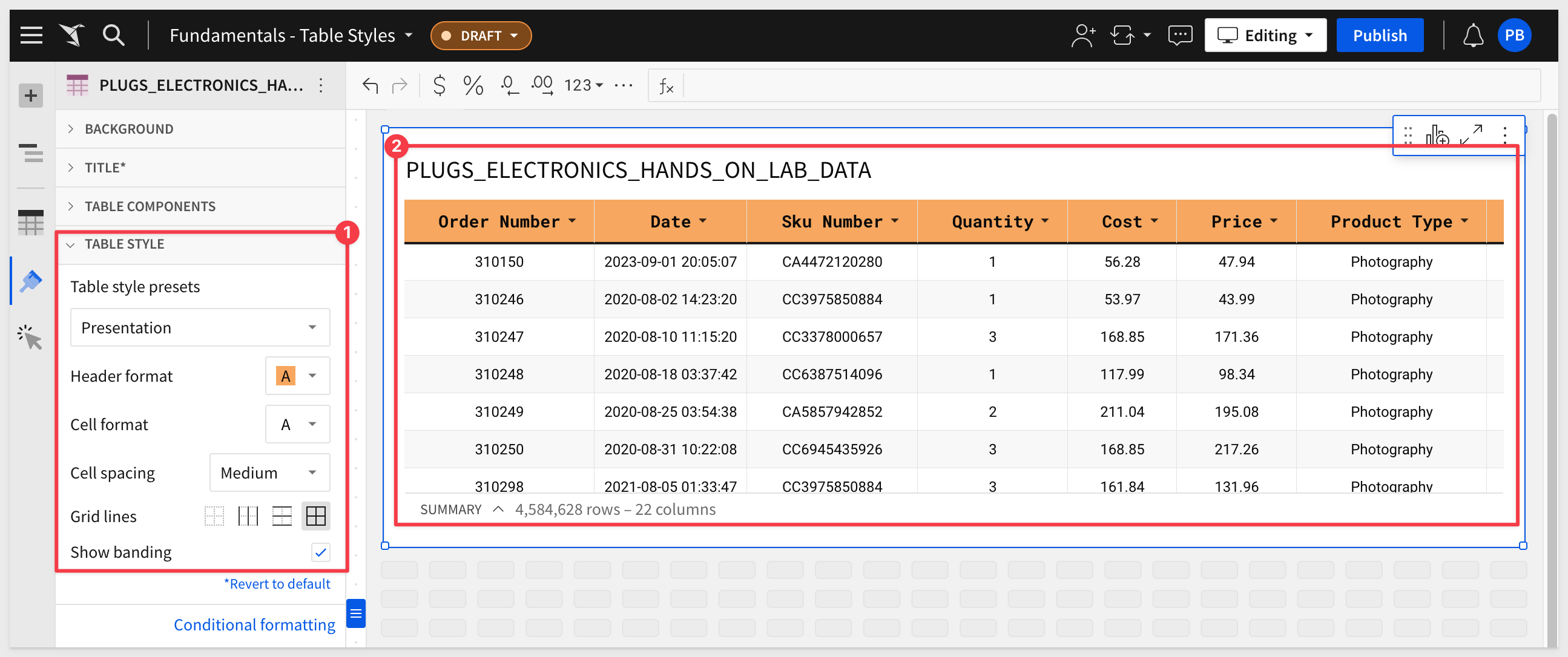
There are many additional customizations you can do to enhance your tables. It is really easy to experiment and see what you can come up with:

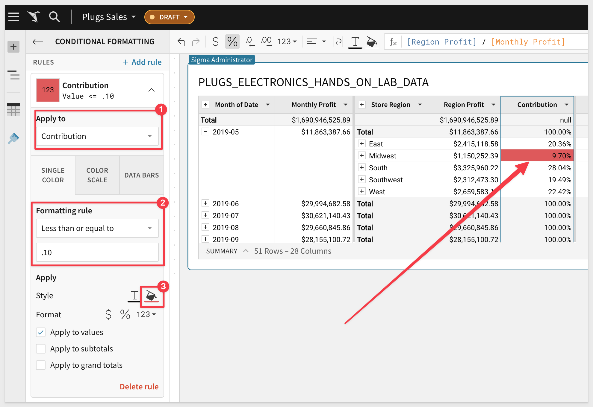
Sigma Workbook Tables can use colors to give the user a more comfortable experience, drawing their eyes to important information through the use of Conditional Formatting.

Using the drop-down on the Contribution select Conditional Formatting. Sigma automatically applies a base color scheme to the column. You can use the Elements Panel to adjust to suit your needs.

In the left-hand pane, select Single Color and set the values as shown below. We can now see which regions had a Contribution lower than 10% in red.

There are many things you can do to enhance your Table; feel free to experiment and see what you can come up with.

Sigma also has the ability to create Summary Values or KPIs across the entire table. At the bottom of the table you will see a line that says Summary which shows the number of rows as well as the number of columns.

At the bottom left corner of the table click on the caret and select the + button.

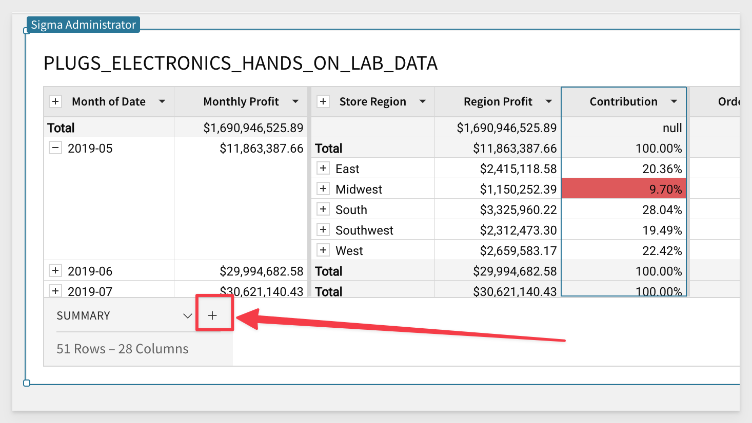
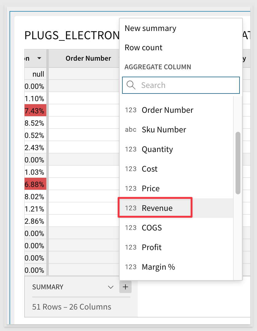
Select the Revenue column. Sigma will automatically sum the column.

You can adjust this formula at any time from the formula bar to be anything you want.

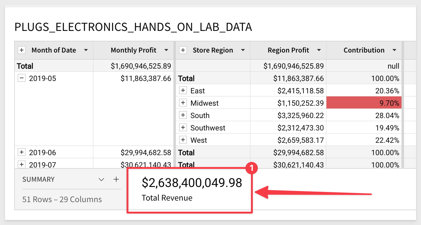
Rename the summary to Total Sales, format it as currency and trim the trailing cents values.

These summary values can now be accessed in any formula (by name) anywhere in the table and can also be leveraged with our KPI visualizations.

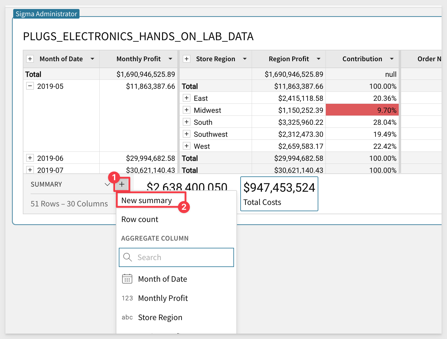
Let's create one more summary value by clicking on the caret ^, and selecting the + button. This time select the Cost column.

Rename this summary to Total Costs and trim the trailing cents.

Let's create one more summary value by clicking on the caret ^, and selecting the + button. This time Select New Summary. This will give us a blank summary which we can write a function for:

In the function bar, enter the formula bar enter:

[Total Sales] - [Total Costs]

Also rename this Summary to Total Profit.

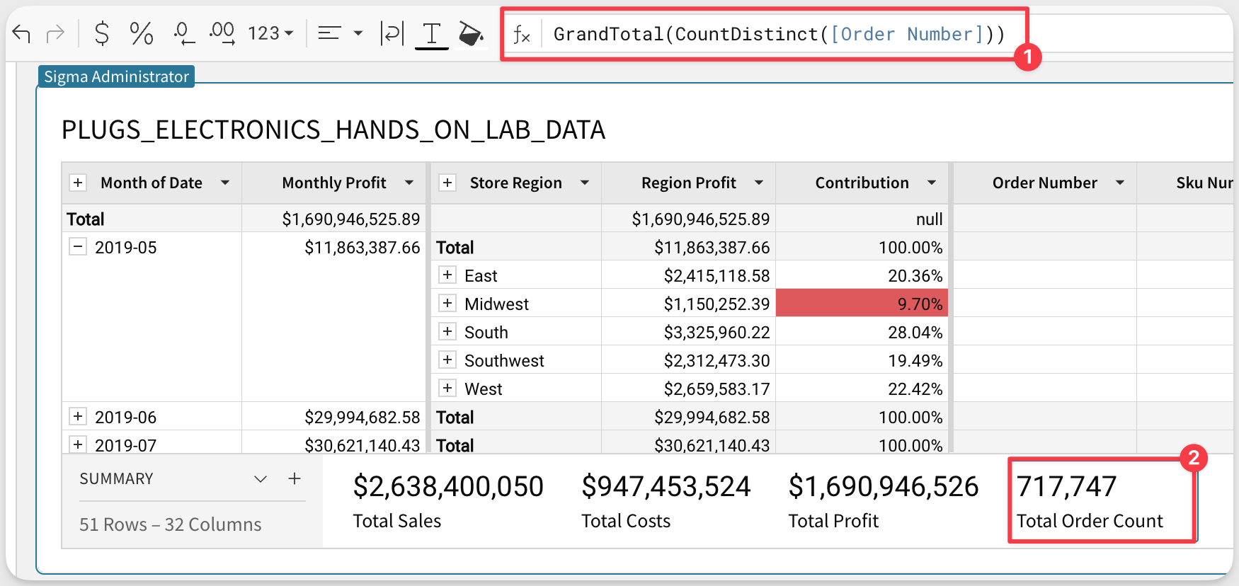
It may also be helpful to have the total number of orders represented in the data. Sigma has a function for that.

Add another New summary and set the formula to:

GrandTotal(CountDistinct([Order Number]))

Rename it to Total Order Count.

Set the format to Number and remove trailing decimals:

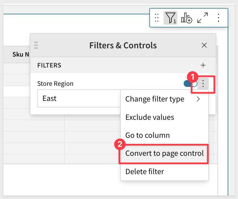
Sigma also has the ability to easily filter table data. Lets filter for only stores in the East region.

Click on the Store Region column and select Filter.

Notice that a FILTERS & CONTROLS panel opens and it auto-populates with the available distinct list of Store Regions.

Also notice that under number 3 there is a small filter icon with a 1 next to it. This lets you know that the table has a filter set against it. This will come in handy to know as you work.

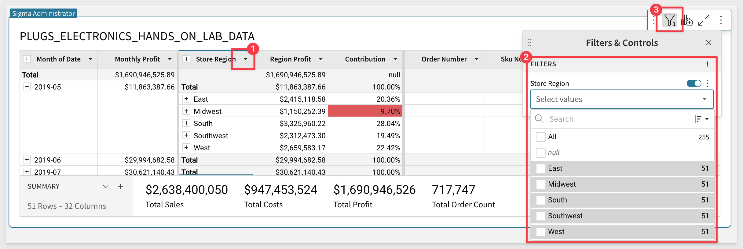
Click the checkbox for East and see the table update for just the East region. The summaries are also updated.

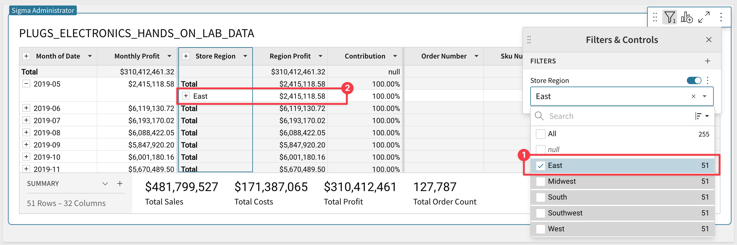
Wouldn't it be great if I could just have this filter as as dropdown on the Page? No problem.

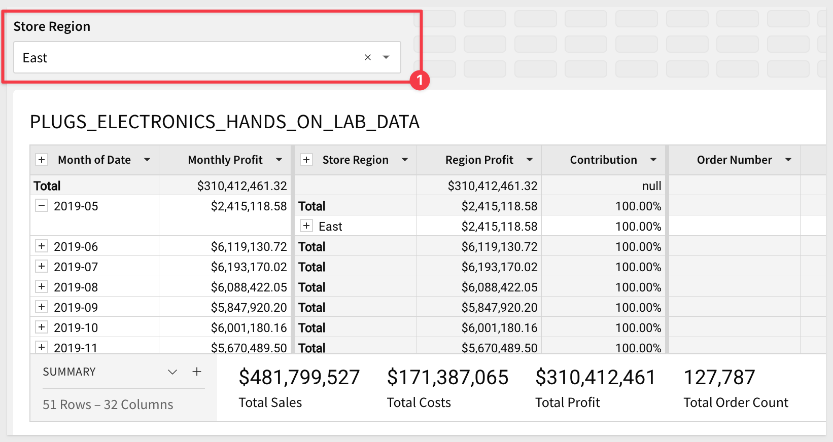
Just click the vertical 3-dots and click Convert to Page Control.

Now the Table can be filtered by using the dropdown filter list as shown below:

You may want a totally different page layout and we will cover that along with more information on page controls in the Dashboard QuickStart.

In this QuickStart we covered how to access sample data to build a table, add new calculated columns, group and filter data and apply conditional formatting and filter the result set.

Click here to move to the next QuickStart in this series.

Additional Resource Links

Be sure to check out all the latest developments at Sigma's First Friday Feature page!

Help Center Home
Sigma Community
Sigma Blog