Skip the ETL pipeline — three production-ready use cases showing how Sigma input tables let users write data directly to the warehouse.
input tables are Sigma-managed warehouse tables, through which users can add their own data and integrate into their own analysis.
When data isn't in the warehouse, it usually requires a cumbersome technical and people process to ETL data into the warehouse. Now users who need to add data to the warehouse are able to do so directly.
Sigma customers already use input tables for:
- Manual data entry of key values
- Analytic Modeling
    <ul>
    <li>scenarios</li>
    <li>forecasts</li>
    <li>territory planning</li>
    <li>sales planning</li>
    <li>supply chain modeling</li>
    <li>categorizations</li>
    </ul>
</li>
For more information on Sigma's product release strategy, see Sigma product releases.
Target Audience
Anyone who is trying to create QS content using Sigma and wants to augment, adjust, interact and create "what-if" scenarios.
Prerequisites
- A computer with a current browser. It does not matter which browser you want to use.
- Access to your Sigma environment. A Sigma trial environment is acceptable and preferred.
- Some familiarity with Sigma is assumed. Not all steps will be shown as the basics are assumed to be understood.
- Downloadable project files discussed later in this document.
- A Snowflake account with the proper administrative and security admin access.
- Microsoft Excel or Google Sheets (for accessing the provided sample data)
What You'll Learn
We will review a few different ways customers are using input tables already and show you how to make them work in your own Sigma environment.
What You'll Build
We will review these three use cases:
<ol type="n">
  <li><strong>Forecasting</strong></li>
  <li><strong>Rapid Data Prototyping</strong></li>
  <li><strong>Territory Planning</strong></li>
</ol>

In our first use case, Paula, the VP of EMEA sales, is running her forecast call, where her country managers each call out the final numbers for the year, and any adjustments that they may want to make.
This has traditionally been done on a spreadsheet that Paula created by merging multiple spreadsheets together.
She's also planning out the next year and adds growth numbers for each country.
The spreadsheet work is a time-waster for her and can also be error prone.
Input tables to the rescue
Open Sigma and create a new workbook.
Change the name of the workbook to Input Table Use Cases.
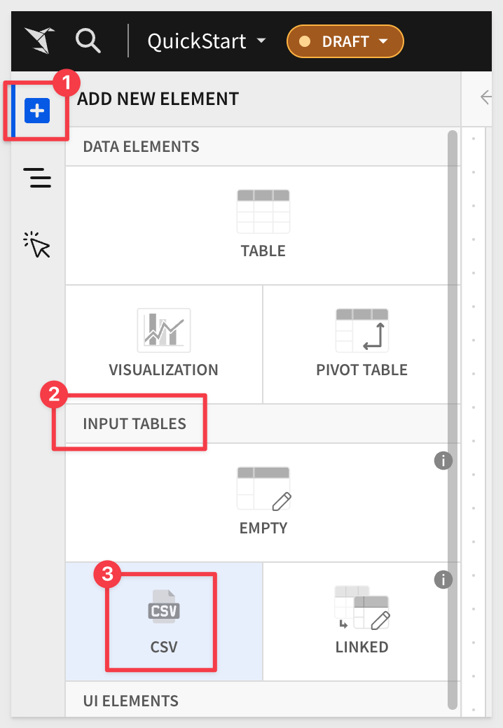
Add a new page to our workbook and rename it to Forecast Adjustment.
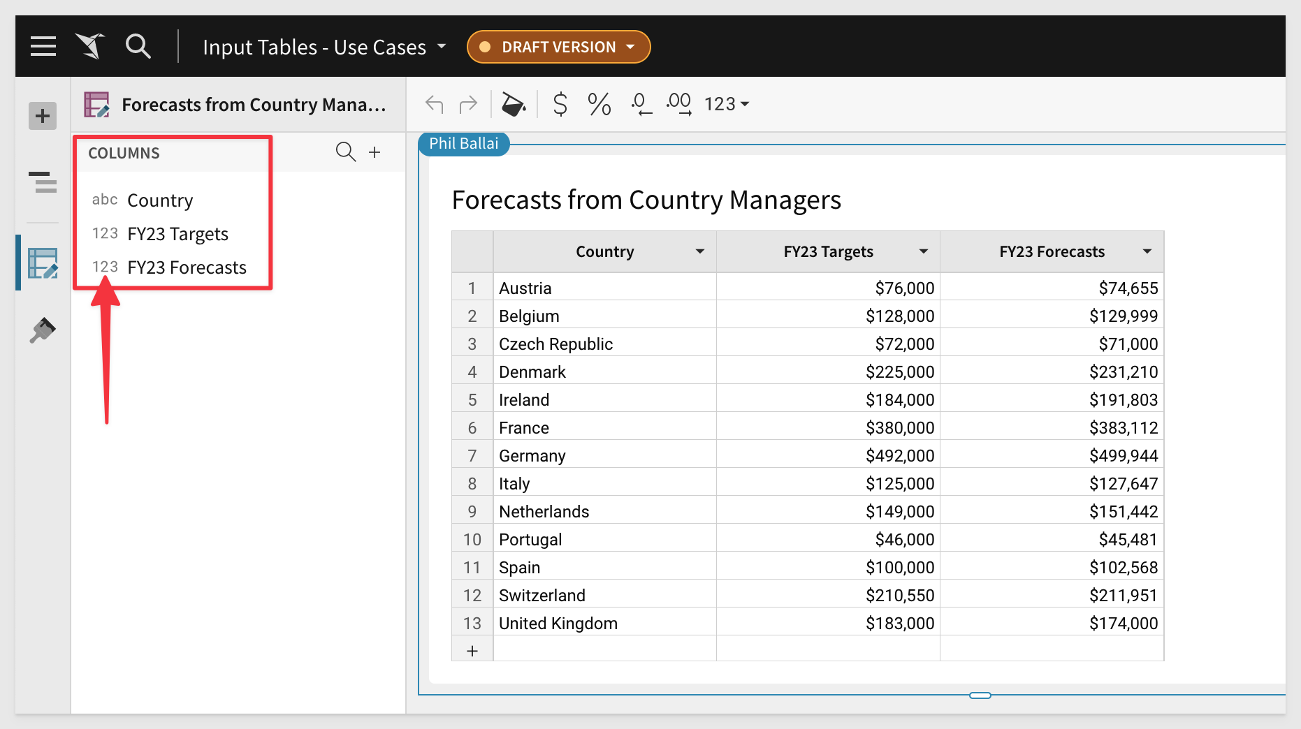
Add a new CSV Input Table to the page and rename it Forecasts from Country Managers:
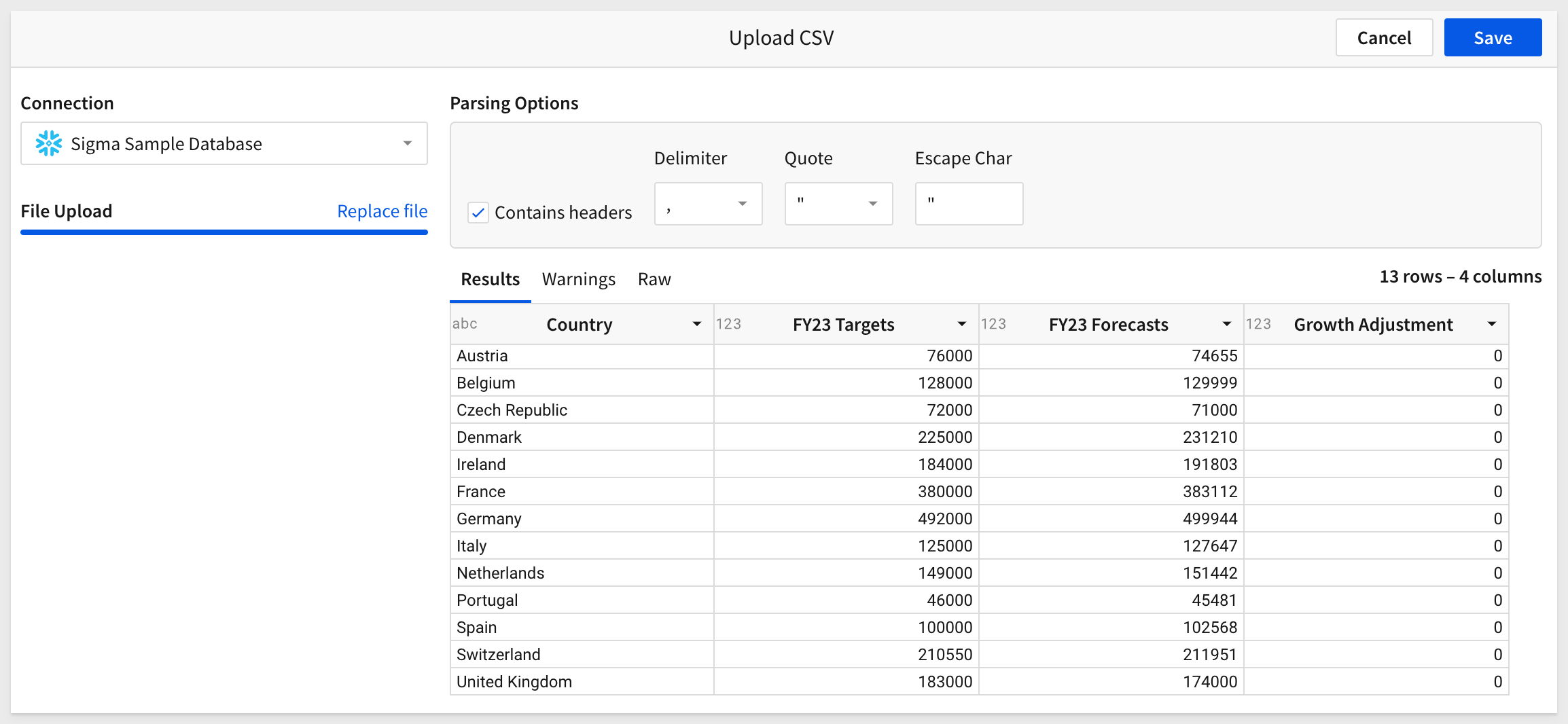
Use Sigma to import the downloaded file, import it and click Save:
Click here for information on setting up Write access.
Rename the new input table to Forecasts from Country Managers.
Notice that Sigma automatically identified the data types for you, saving time.
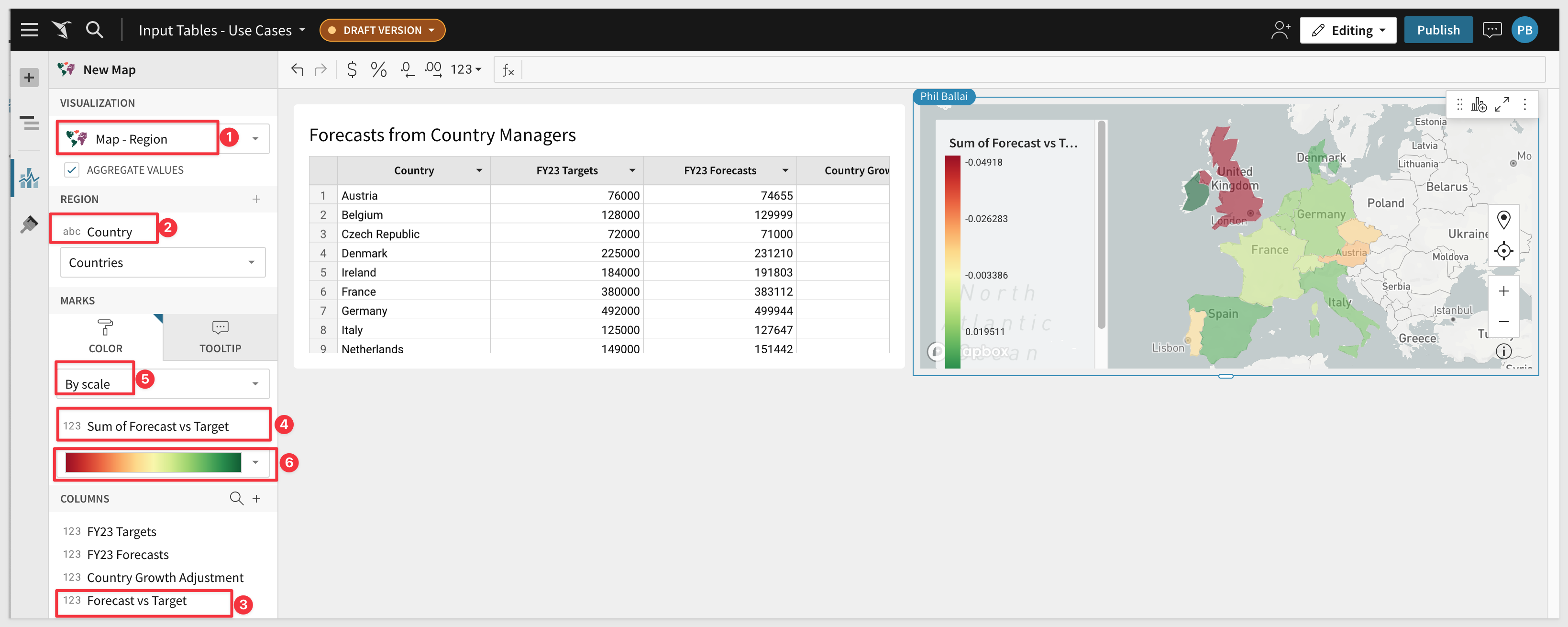
Add a new Visualization to the page, use the input table as it data source, set it to Map - Region and drag the Country column up the Regions.
We want this map to show different colors for FY23 Targets vs FY23 Forecasts, so we need to add a new column to the data that represents this calculated value.
In the Element Panel / Columns click the + icon and select new column.
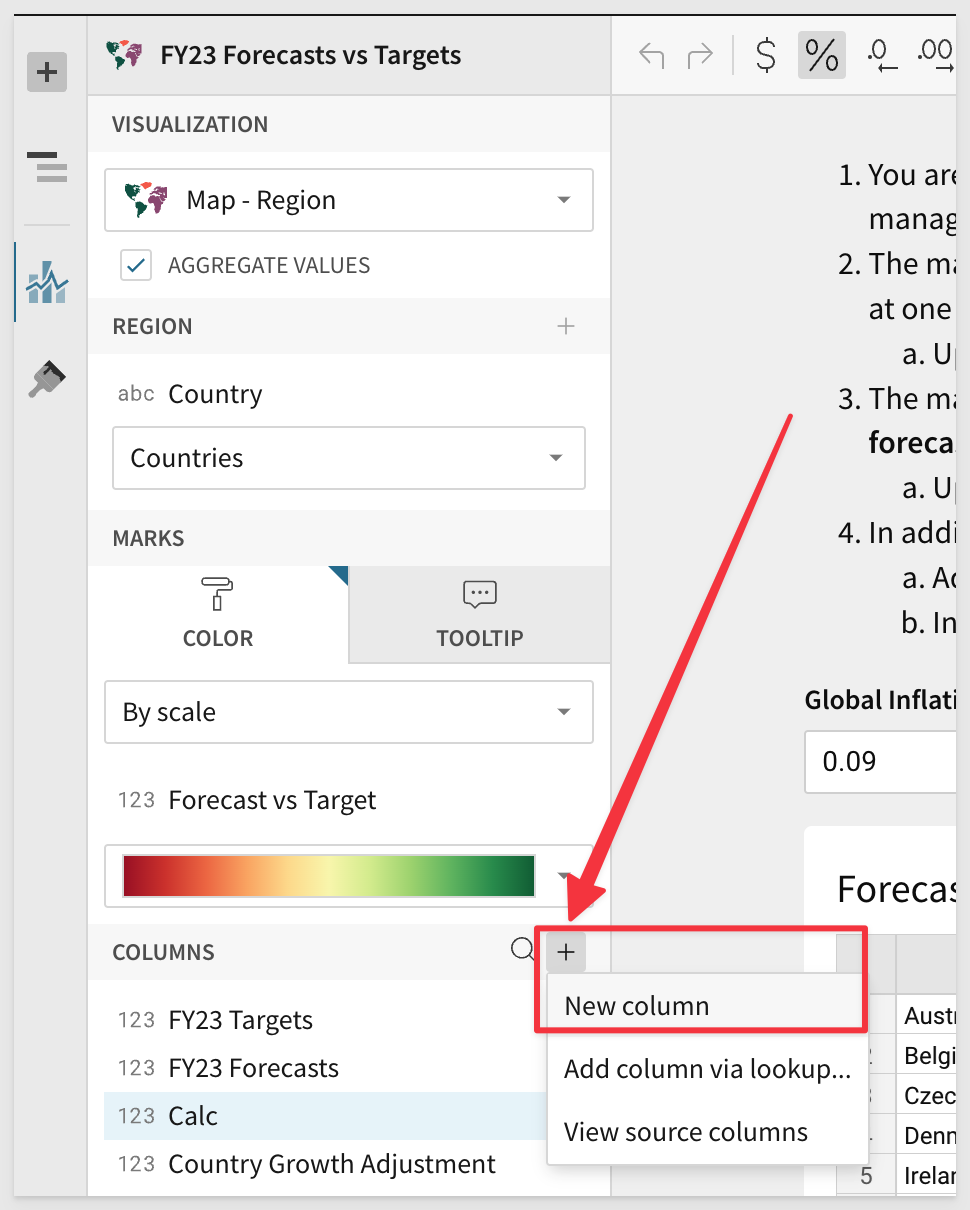
Rename the column to Forecast to Target and set the formula to:
(([FY23 Forecasts] - [FY23 Targets]) / [FY23 Targets])
Adjust the element panel, so that the map appears as shown below:
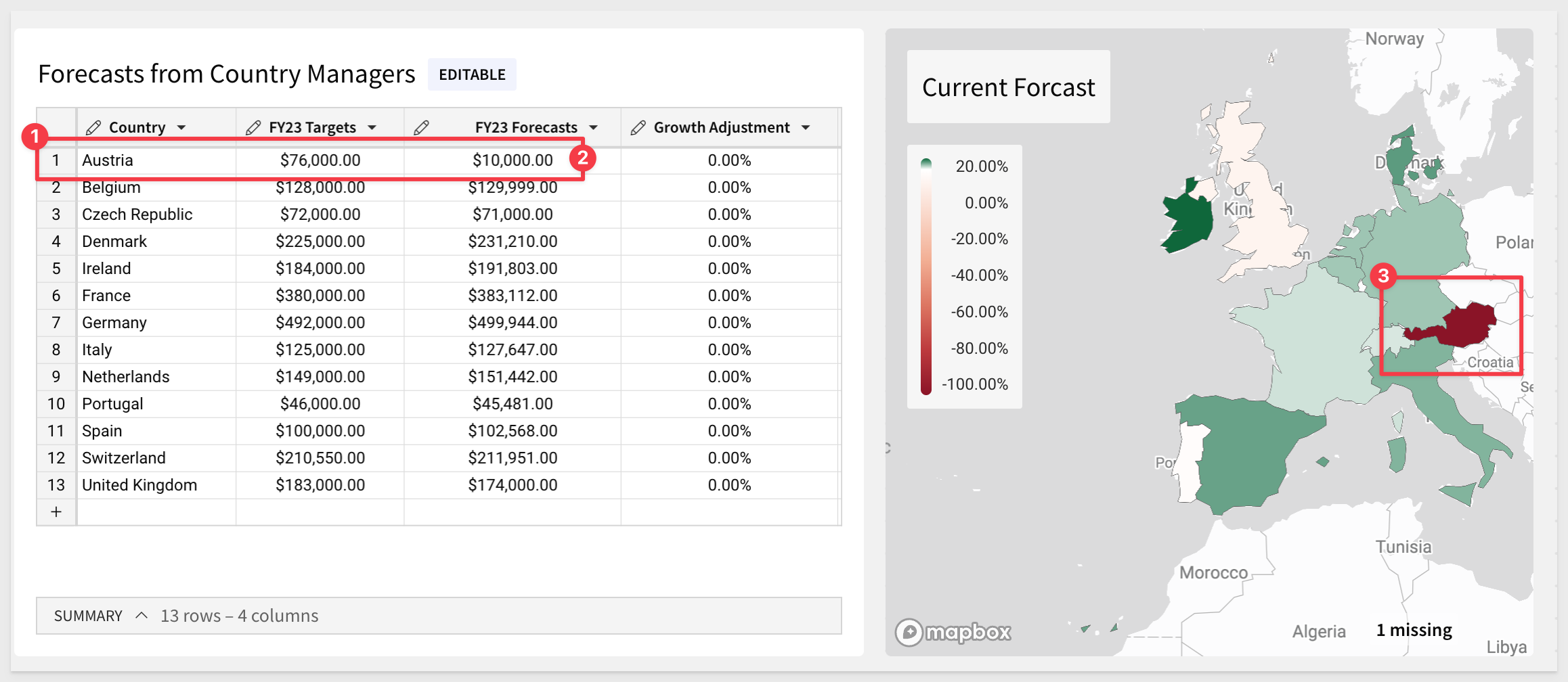
The manager in Austria tells you she's cutting her forecast down to $10k because there was a strike at one of the factories.
Update the input table and see the map change.
Change the FY23 Forecast value for Austria down to $10K and hit Enter.
The map changes automatically to reflect this revision.
Real-time modelling
Paula wants to make her own adjustments after the call and wants to be able to just experiment with making adjustments while considering the impact of small changes in a visualization before making a final decision.
Bar chart
Lets add a bar chart to give Paula the visualization she is wanting, and start by comparing the FY23 and FY24 forecasts (by country).
Add a visualization and configure it as follows:
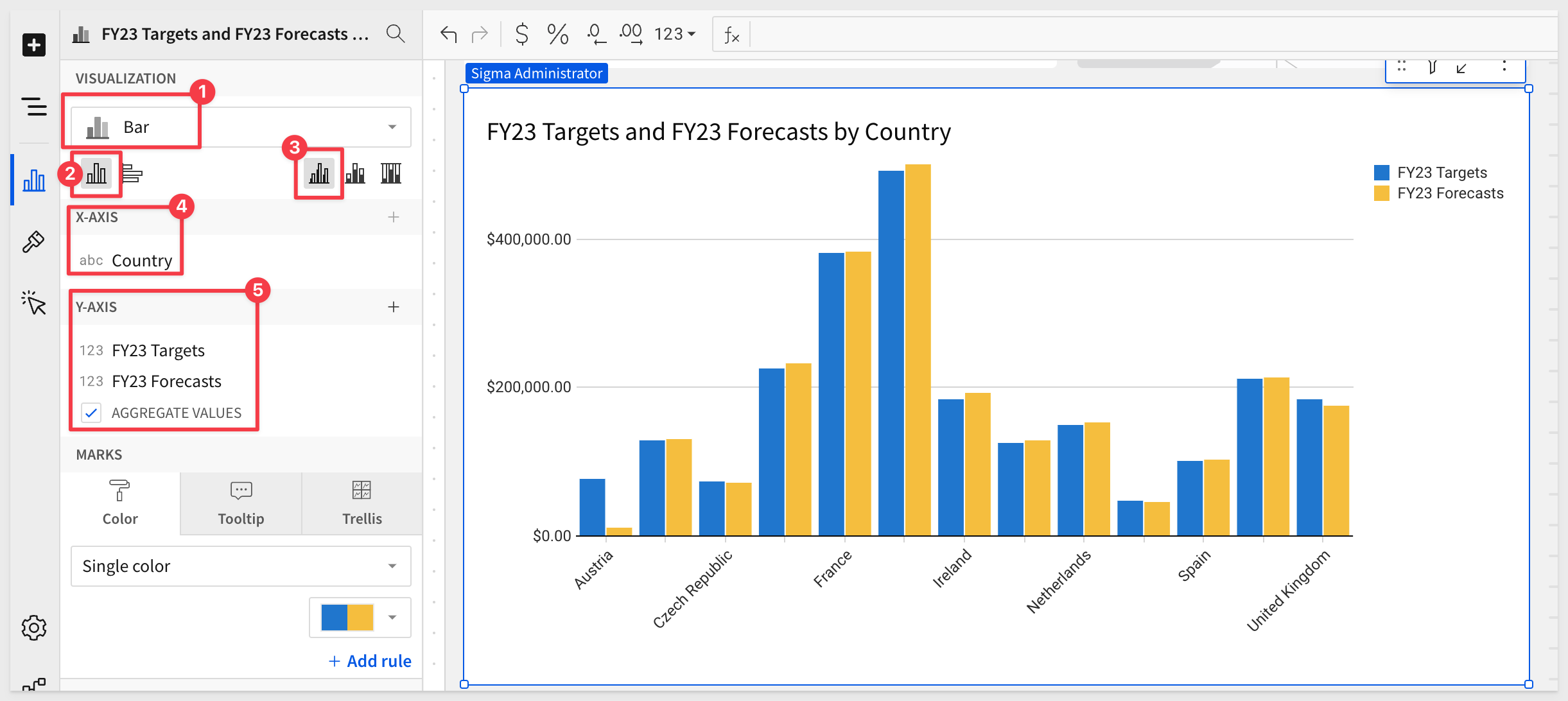
Lets add the Growth Adjustment column to the Y-Axis. At the moment, all the values in this column are zero and that is fine, we will adjust the formula.
We want this new bar on the chart to show the FY23 forecast after the growth adjustment is made in the input table. In this way, Paula can quickly see how a small percentage gain (or loss) will impact the country forecast.
Set the formula bar for this new column to:
[FY23 Forecasts] + ([Growth Adjustment] * [FY23 Forecasts])
Rename the new Column to Paula's Adjustment.
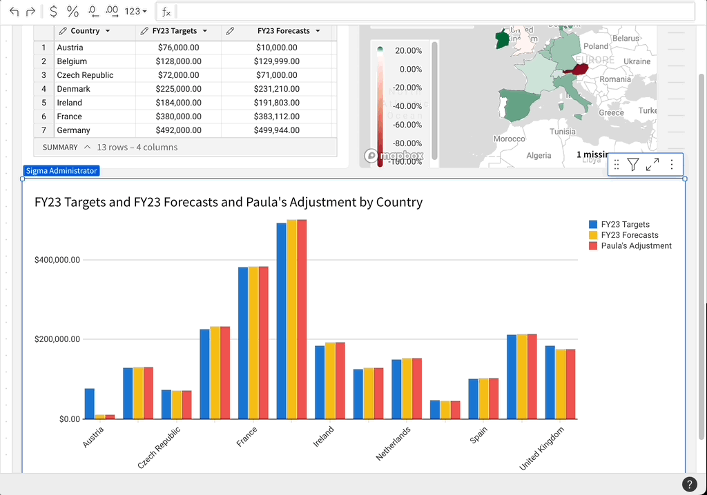
Paula has done some reasearch and thinks that the strike in Austria is not going to happen. She also has been speaking to a large customer in Austria and found that a very large order is coming in that is not forecast.
She reverts the FY23 forecast back to $74655 and also adjusts the growth to 50%, so she can see the impact:
In our second use case, Lucy is a merchandiser at a brick and mortar (B&M) electronics retailer.
She's launching their online store which is powered by Shopify.
Although their B&M data is in the warehouse, the Shopify data is too new and hasn't gone through the modeling process, which takes time.
She can't wait 6 months and has to know now how the new online store is doing.
She has the Shopify data in google sheets where she's been playing around with it. But, it only shows part of the picture.
She needs to see the data from B&M against Shopify in real time.
Sigma allows Lucy to copy and paste the Shopify data into an input table and then is able to compare online vs B&M sales by category and SKU.
This informs her about the strengths and weakness of the online business vs the established B&M, right away.
How to build it:
Open the downloaded file in Excel (or Google Sheets). There should be 5 columns and 82 rows.
We will copy this data into a Sigma input table later.
Add a new page to our Sigma workbook, and rename it to Rapid Data Prototyping.
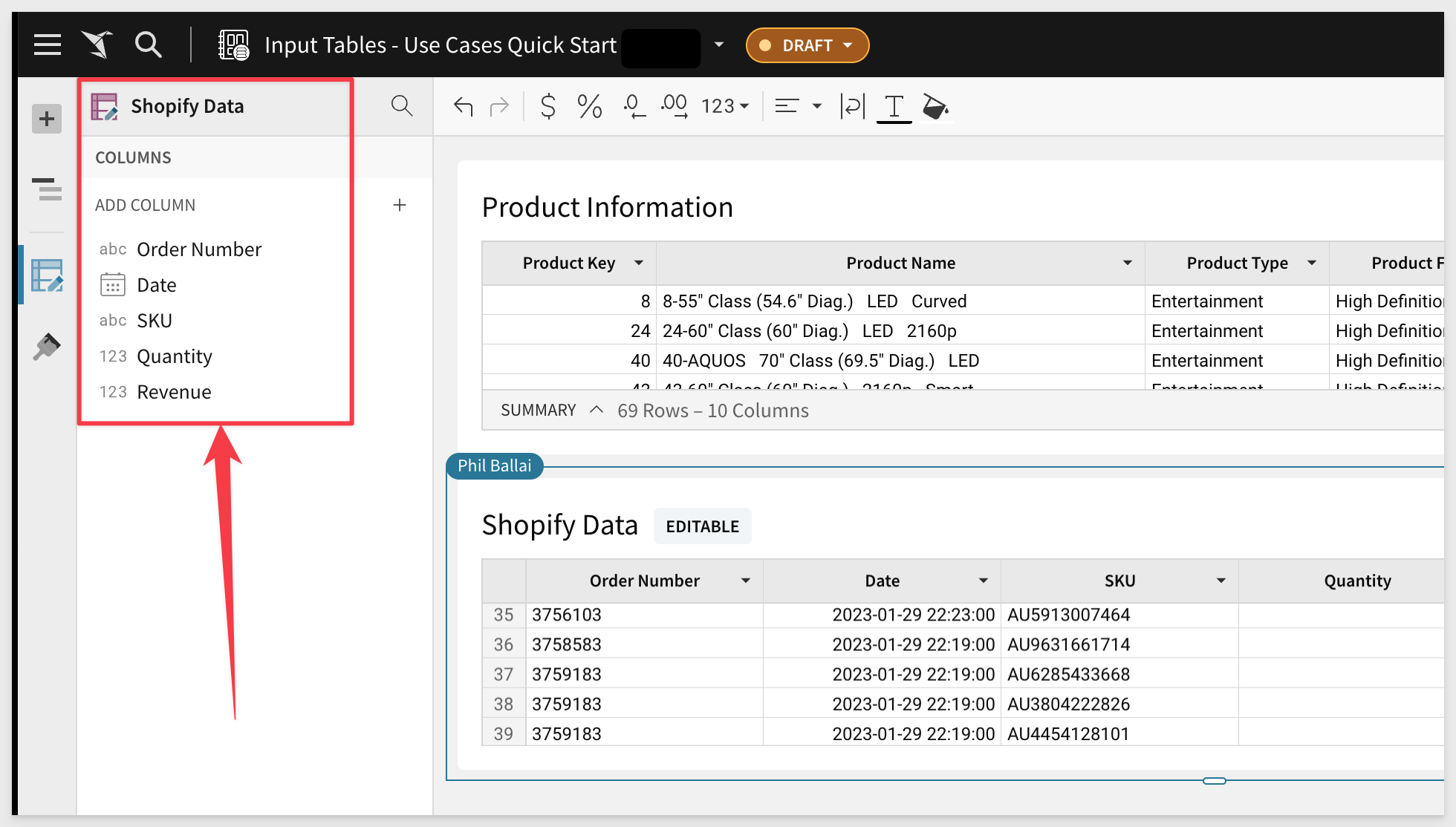
We will add two tables from the warehouse to the page. One for Product Information and another for Brick and Mortar Sales.
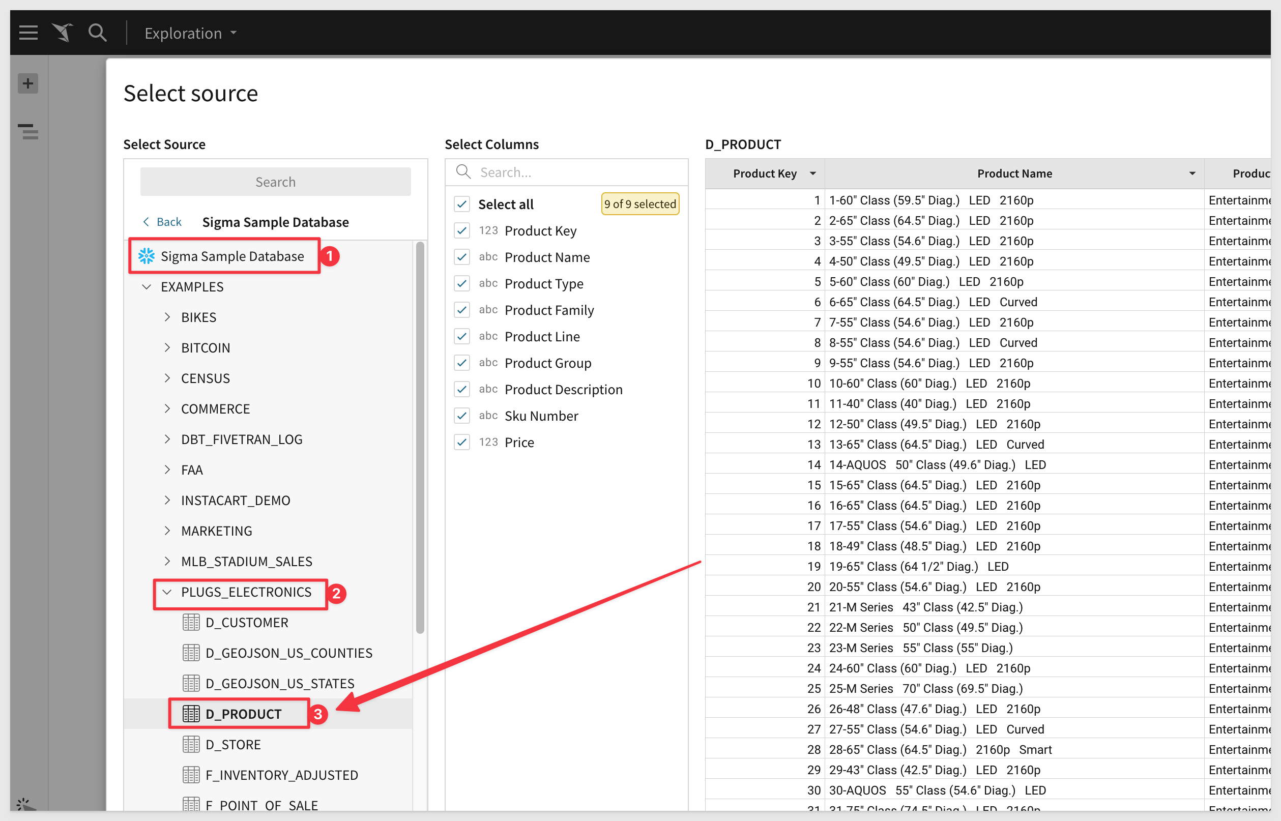
For Product Information we will use the Sigma Sample Database and the D_Product table as shown.
Rename the table to "Product Information".
Create a second workbook Page and rename it Data. We will use this page to hold master reference data that will be reused for this use case and the later ones too.
On the new Data page, add a new table as shown:
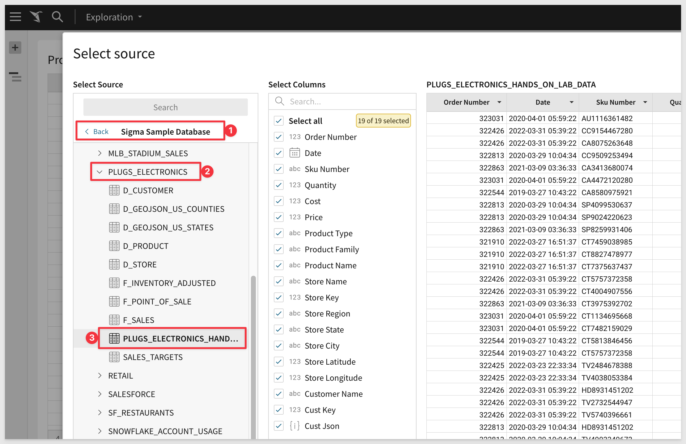
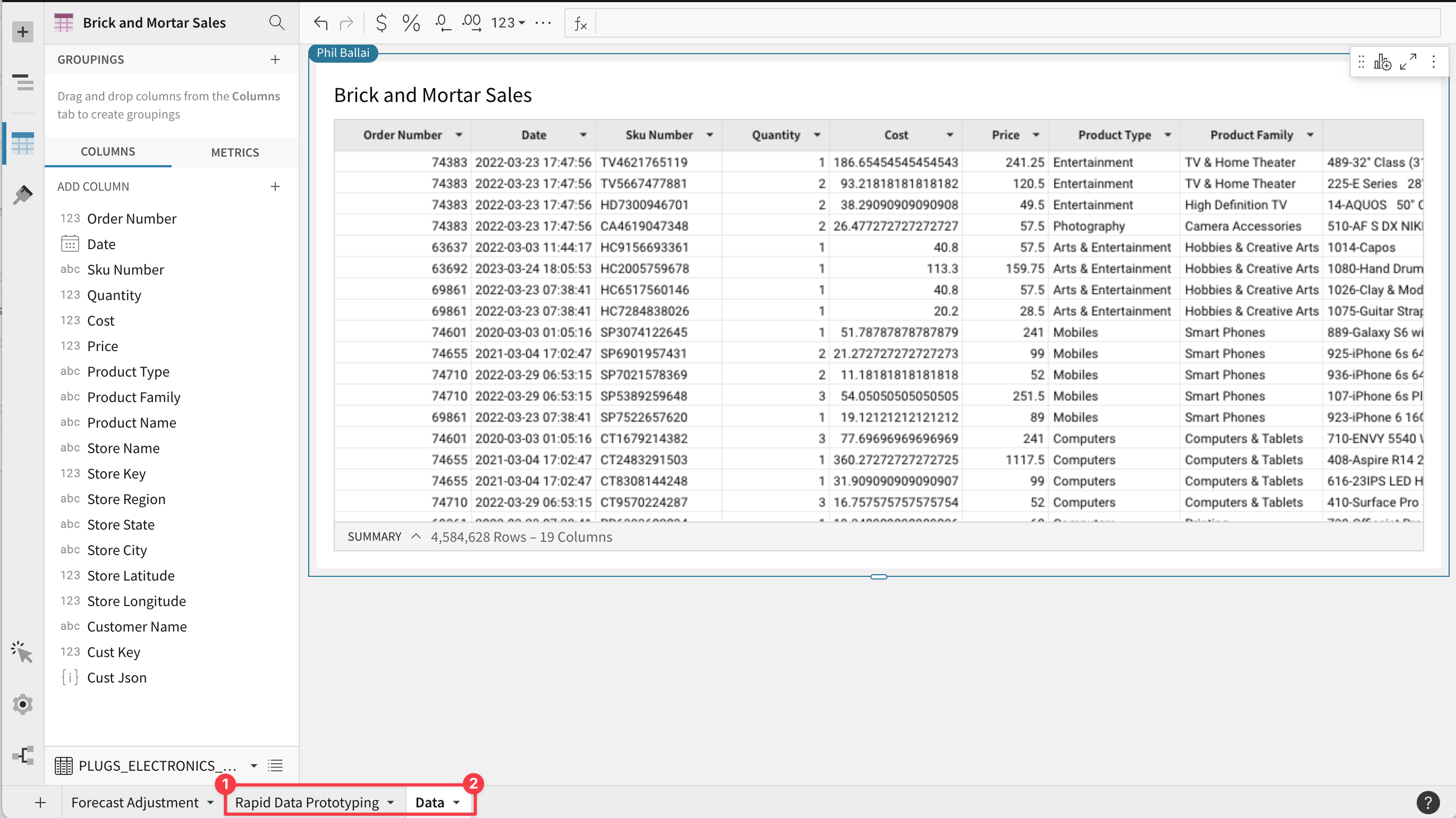
Rename the table to Brick and Mortar Sales.
At this point your workbook should look like this:
Return to the Rapid Data Prototyping page.
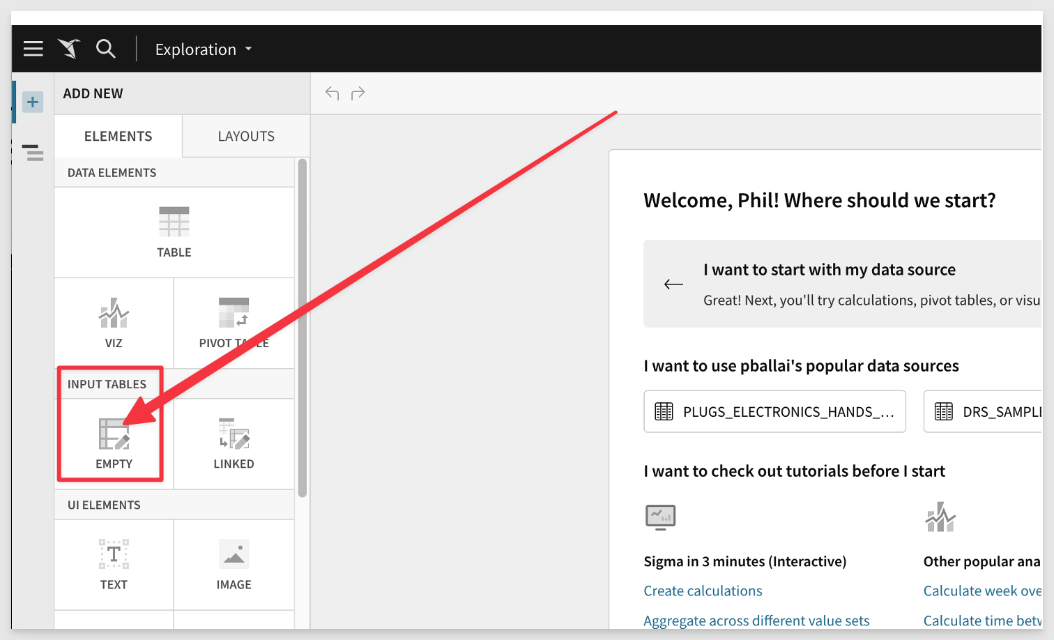
Add a new Empty input table to the Page.
Use the Sigma Sample Database.
Rename the new input table Shopify Data.
Copy all rows and columns from the downloaded Excel file and paste them into the new input table as we did in the first use case.
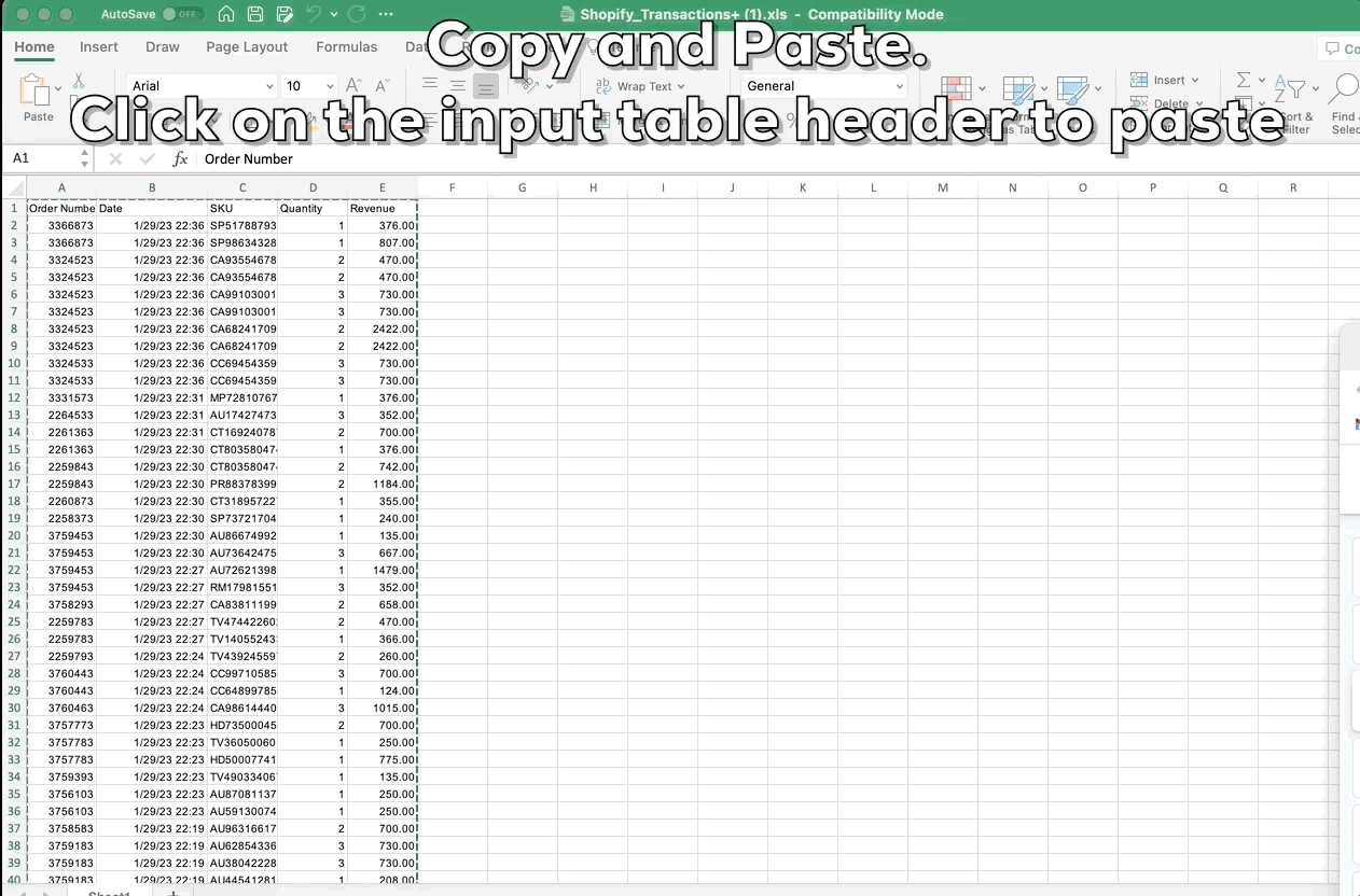
The column headers are automatically set by Sigma.
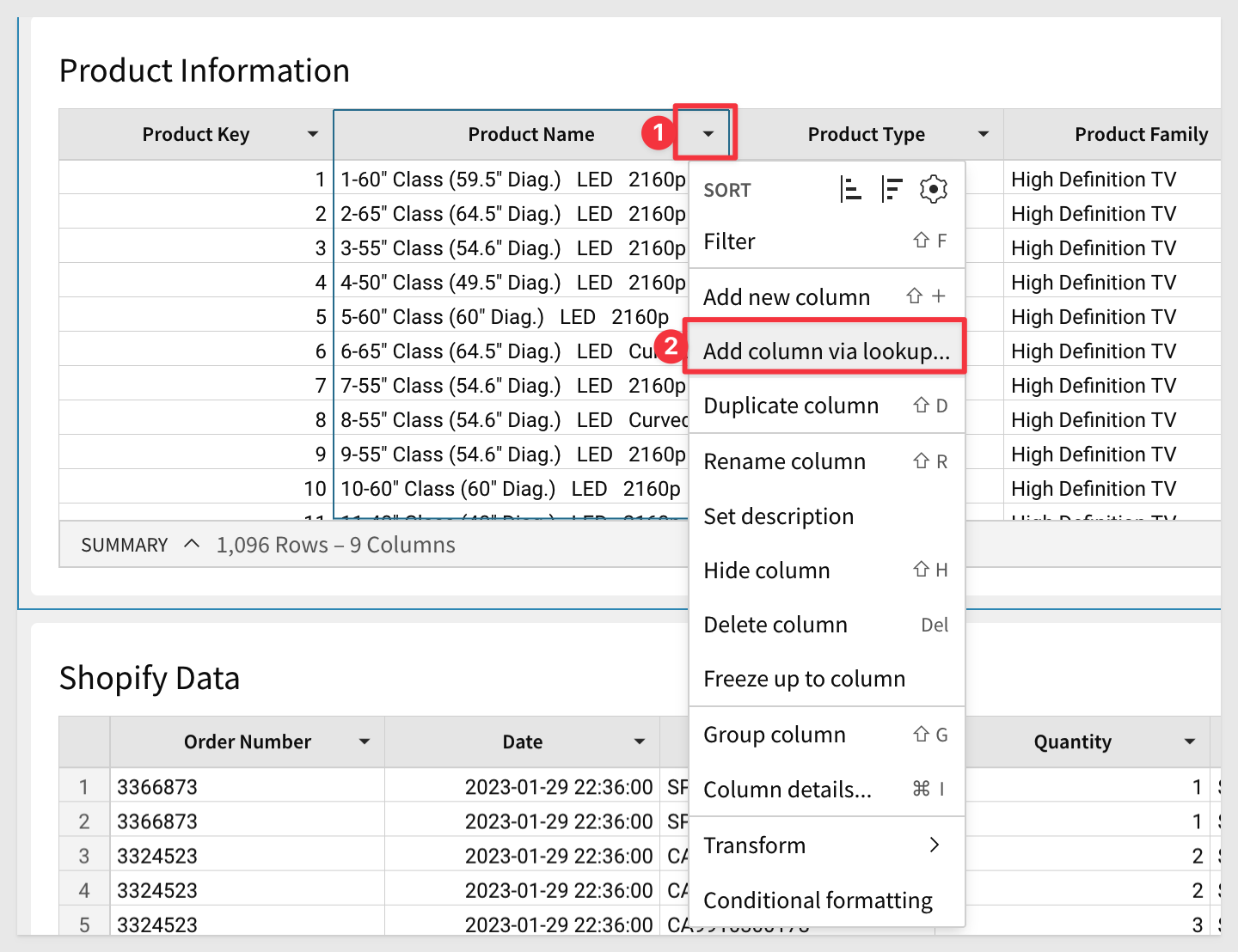
Now that we have the B&M and the online product details, we want to be able to compare them.
In the Product Information table, click the Sku Number column drop and add a Column Lookup.
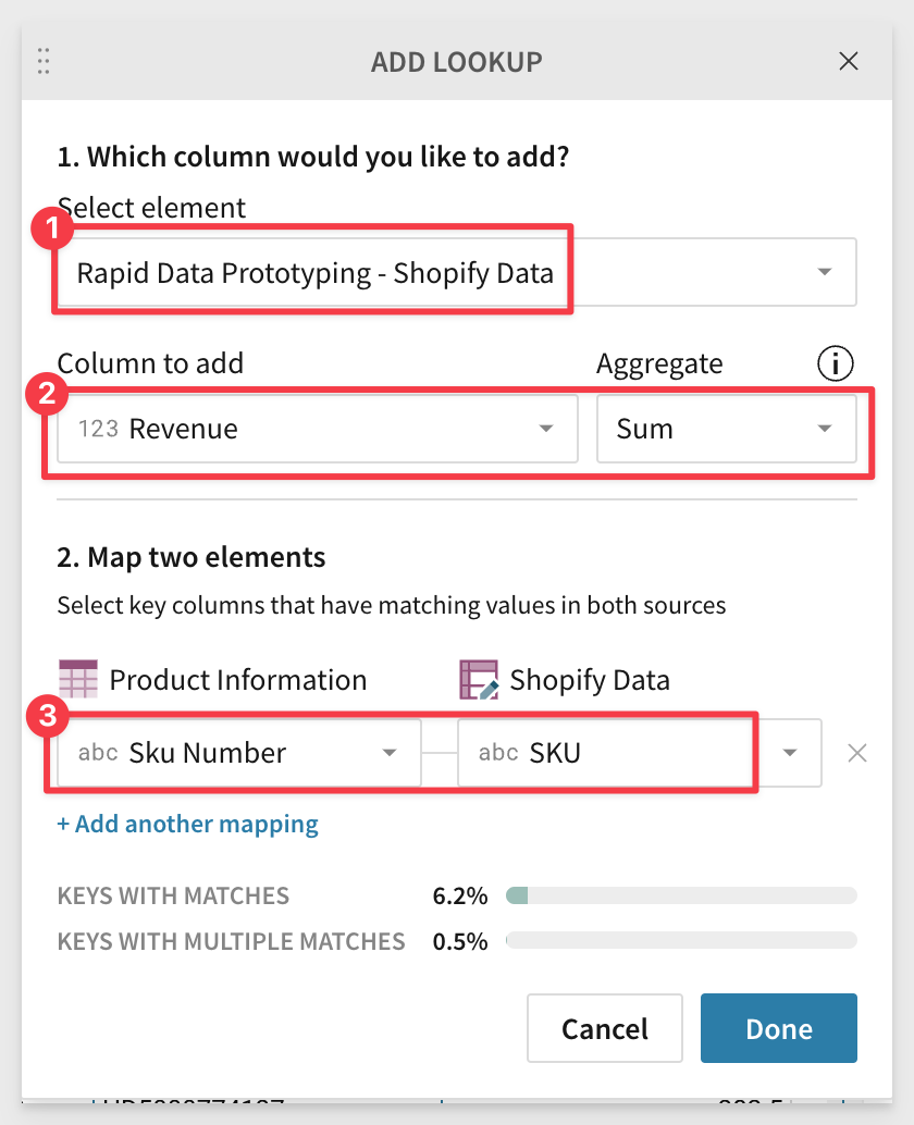
Configure the Lookup as shown:
Many products have not been sold online yet, so right click on the first cell with a null and select Exclude null:
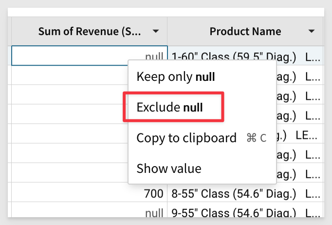
Rename this new column Shopify Reveune and format it as Currency.
Add another new column and use the same workflow.
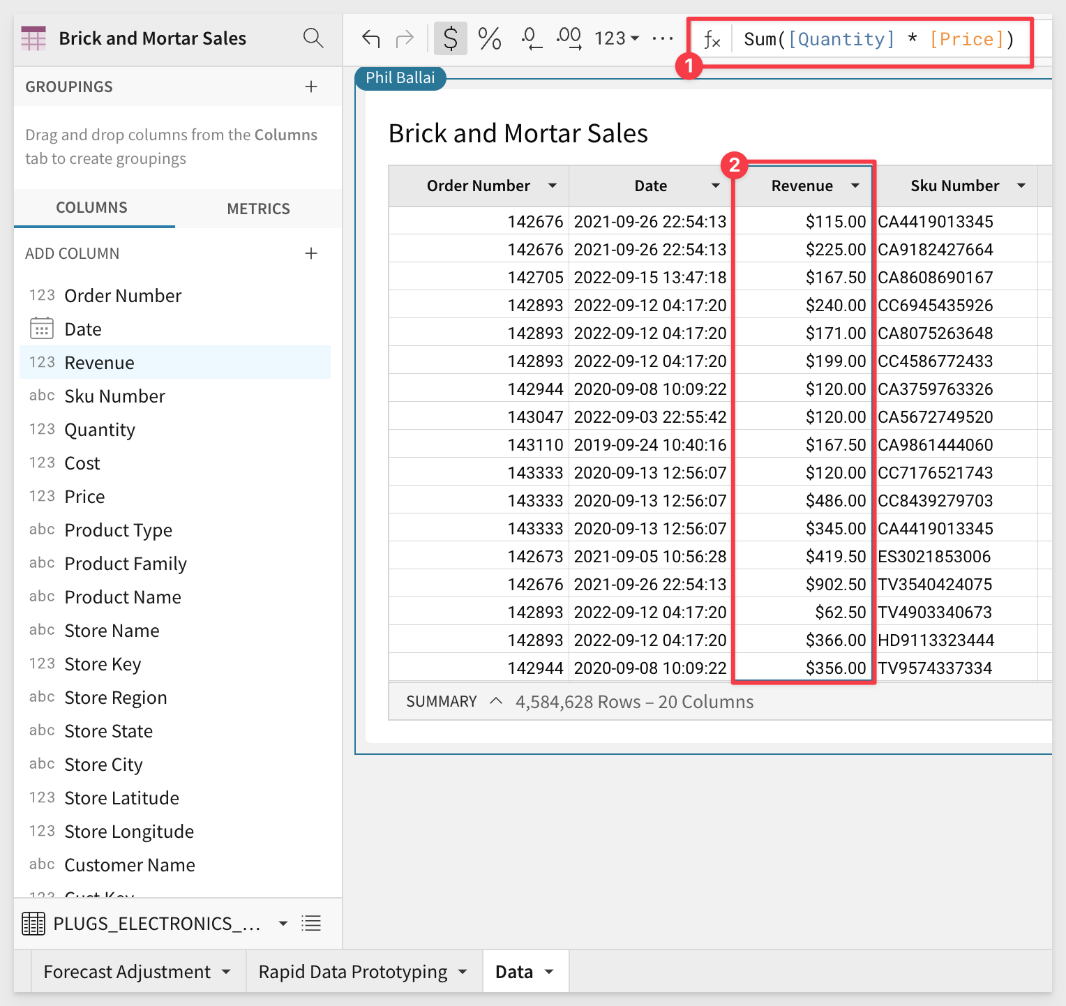
This time we want to pull in the revenue from the B&M table. However, the column Revenue does not exist in the warehouse table Brick and Mortar Sales, so we need to add that first.
Click on the Data page tab and add the new column to the Brick and Mortar Sales table.
select Add a new column and set the formula of that column to (it does not matter the order of the columns in this case):
Sum([Quantity] * [Price])
Rename the new column Revenue and set the format to Currency.
Now we can add a new column to the Product Information table called B&M Revenue using the same workflow for Add a new column via lookup...:
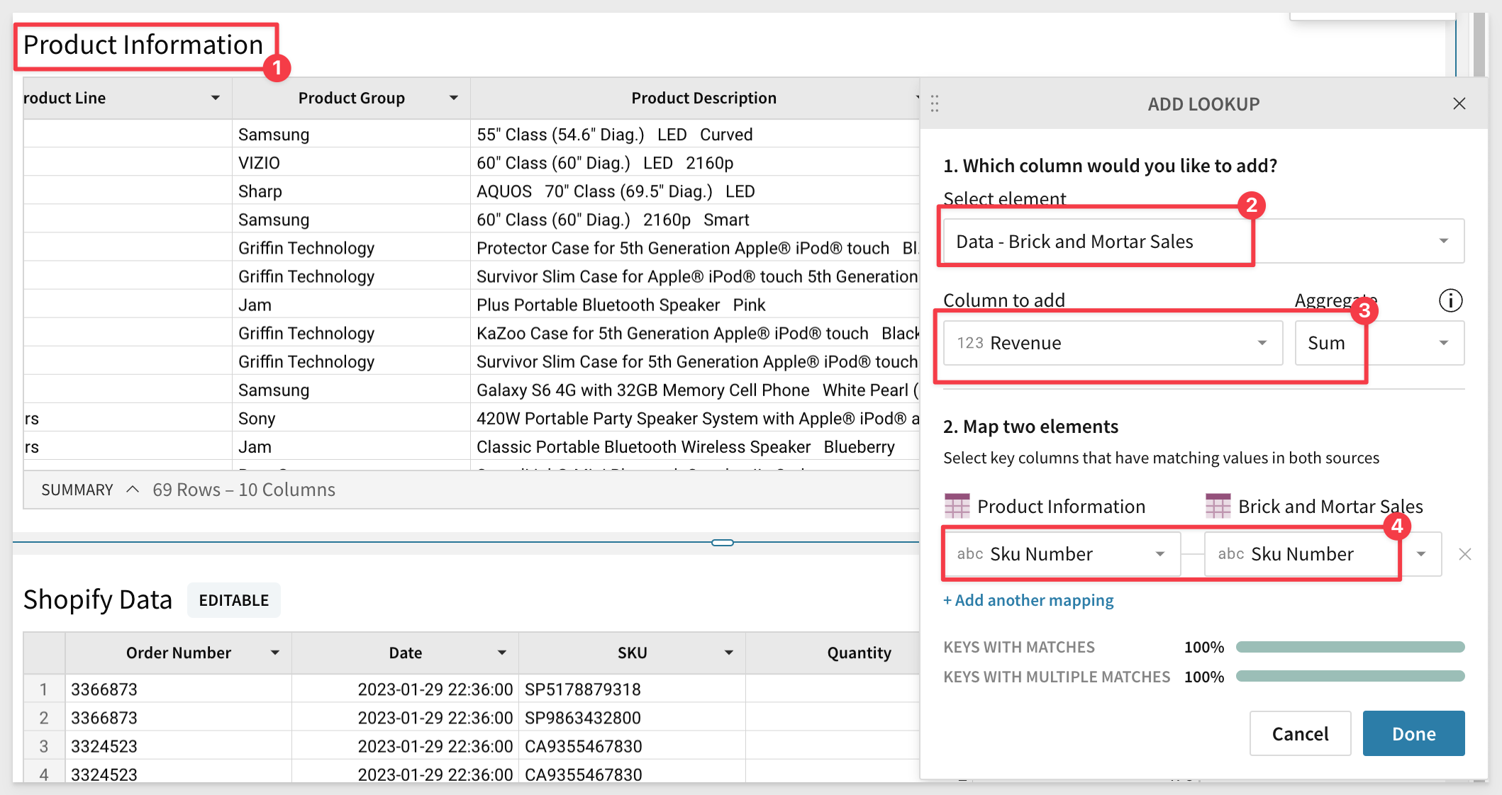
Rename the new column B&M Revenue.
Now that we have the data ready we want to add a new Visualization (Bar Chart in this case) to compare the revenue streams by category for B&M vs. online.
Add a Child Element / Visualization (from the Product Information Table) and set the X and Y axis as shown:
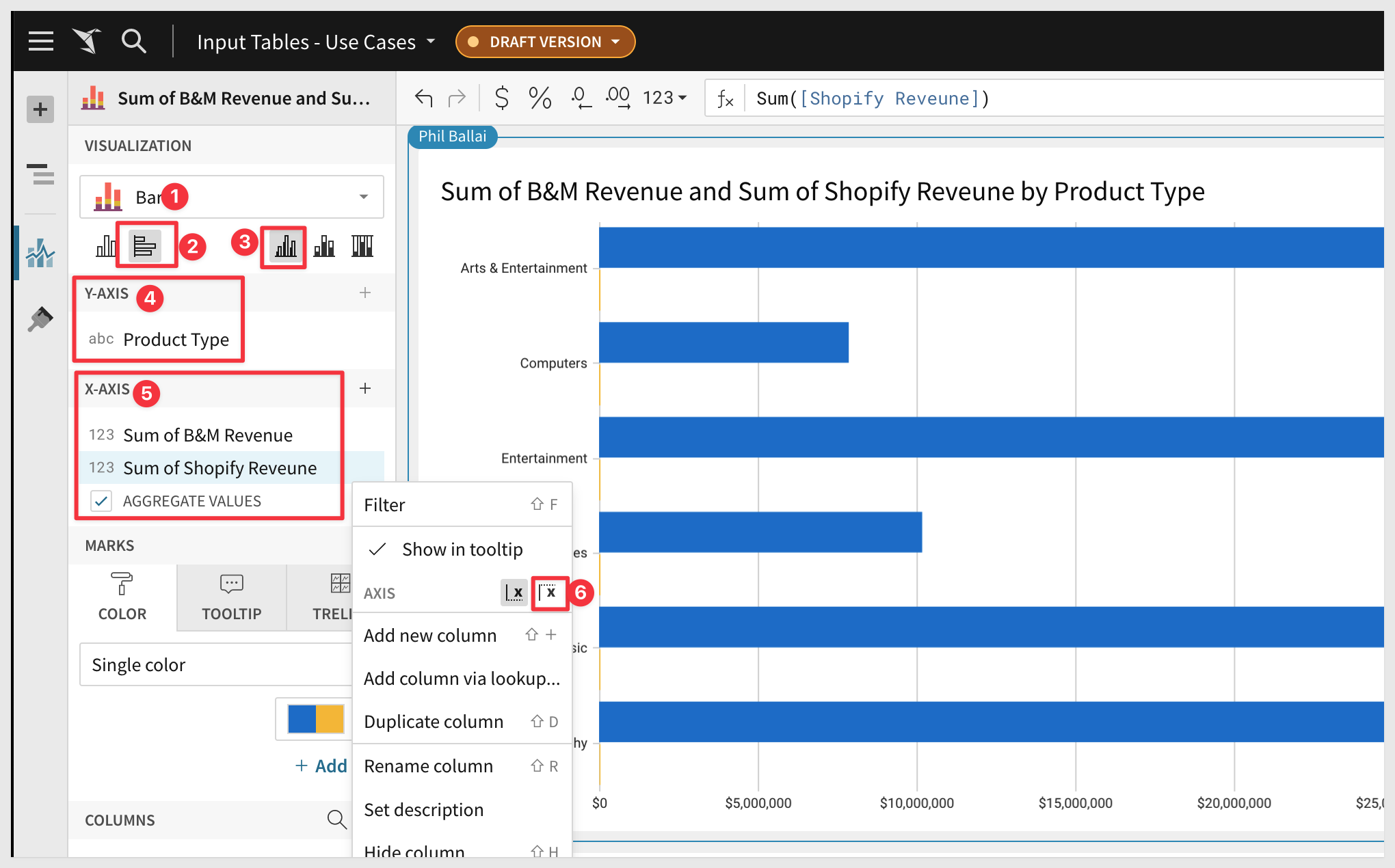
Doing a tiny bit of additional clean-up, we have our chart:

What the chart shows is the relative strength of in-store sales vs. online for each category.
Lucy (our merchandiser) can begin to see which catagories are not selling well online or where to invest more marketing dollars.
This next use case is a bit more sophisticated, using Linked input tables and data validation to allow the user to make on-the-fly adjustments to a sales territory.
Mike, is VP of Sales for the US. His company has grown quickly and the regions need to be rebalanced.
Using Salesforce data in Snowflake, he's able to leverage the power of Sigma and see that the West region has brought in the most revenue.
Specifically, California sales are leading the charts.
Using a linked input table, Mike can dynamically get a list of states and regions based on the latest assignments.
This allows Mike to experiment with the re-balancing, instantly seeing how revenue would change by region based on the new mapping.
The final build will look like this:
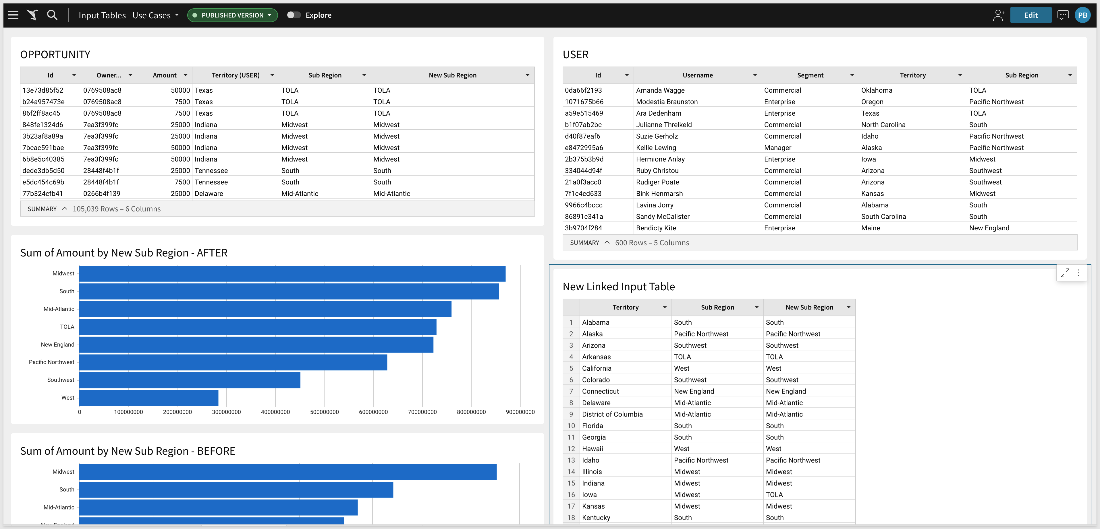
In Sigma, create a new Page in our input tables Demo workbook and rename it Territory Planning.
We will add tables to the page from the Sigma Sample Database / Applications / Salesforce data source.
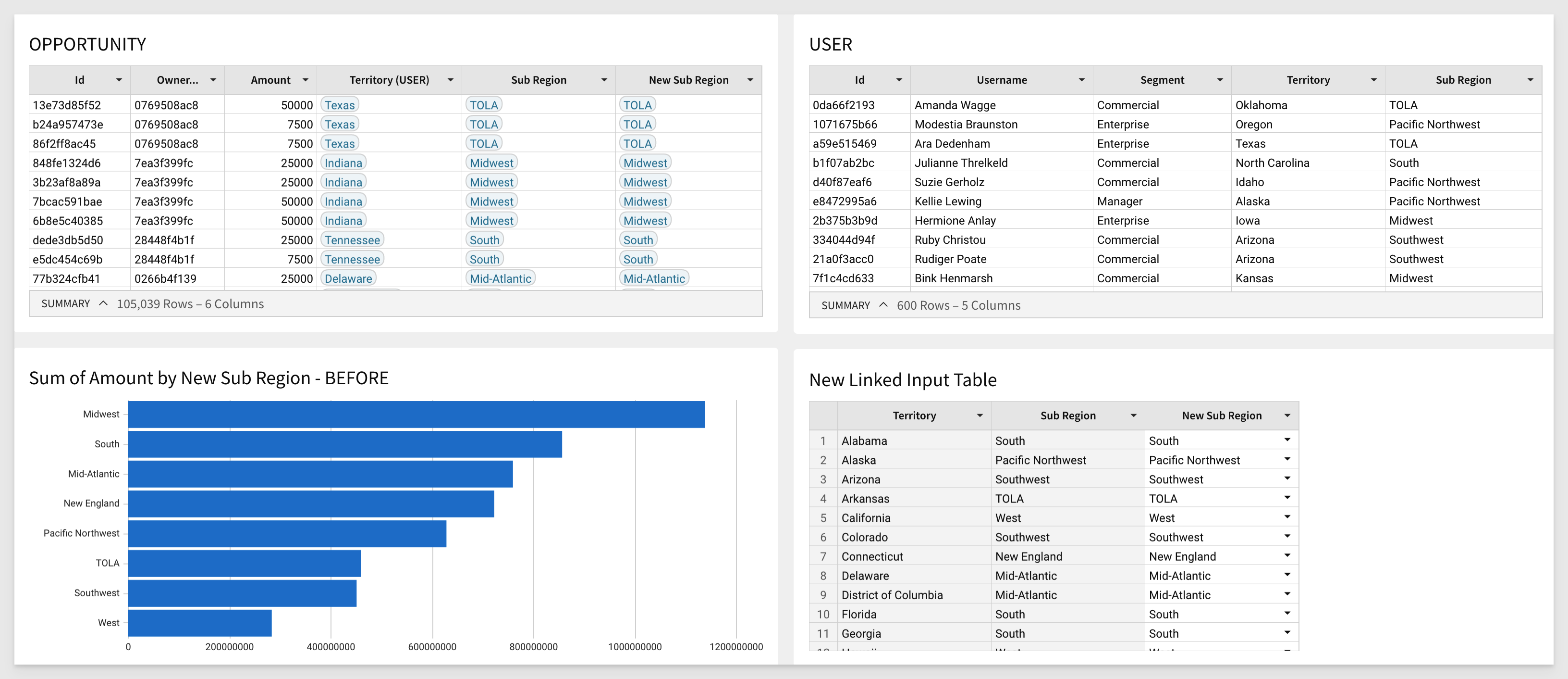
Add USERS, culling the column list as shown:

Add OPPORTUNITY as shown:
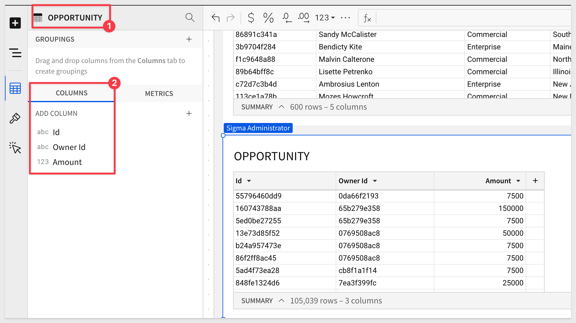
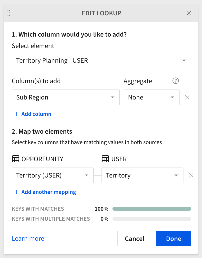
Since the Opportunity table does not contain Region or Territory we we add them using Sigma's Lookup function.
From the Opportunity table and click Add a new column via lookup as shown:
a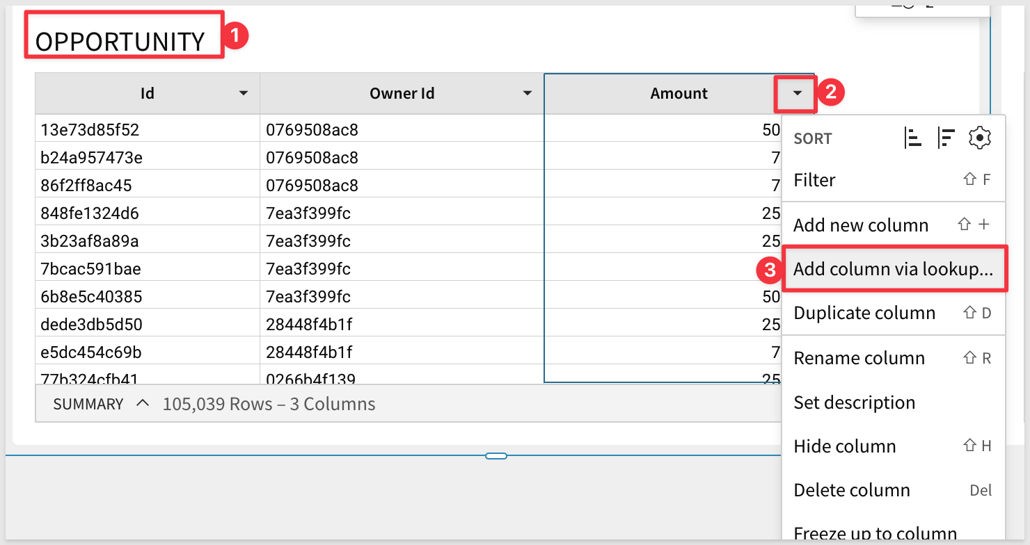
...and configure it as follows:
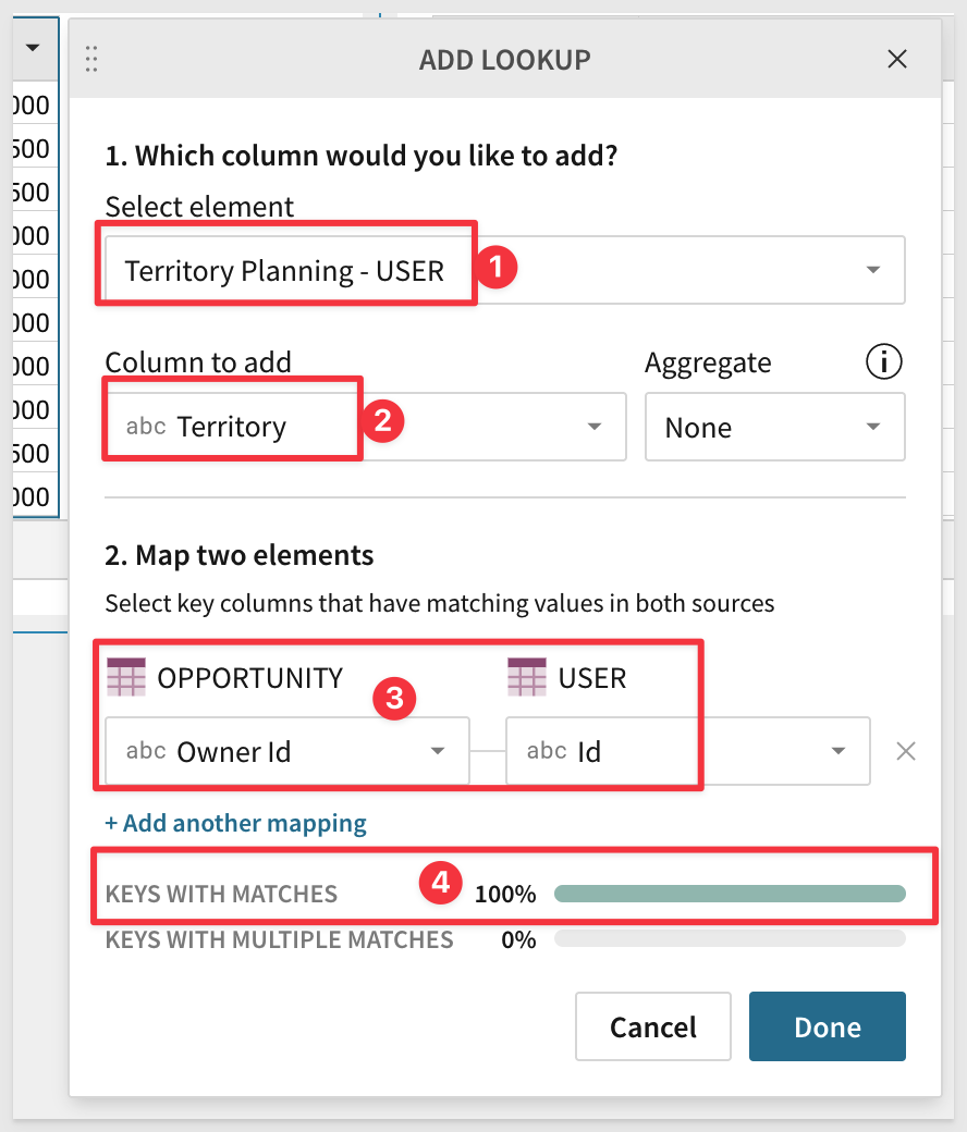
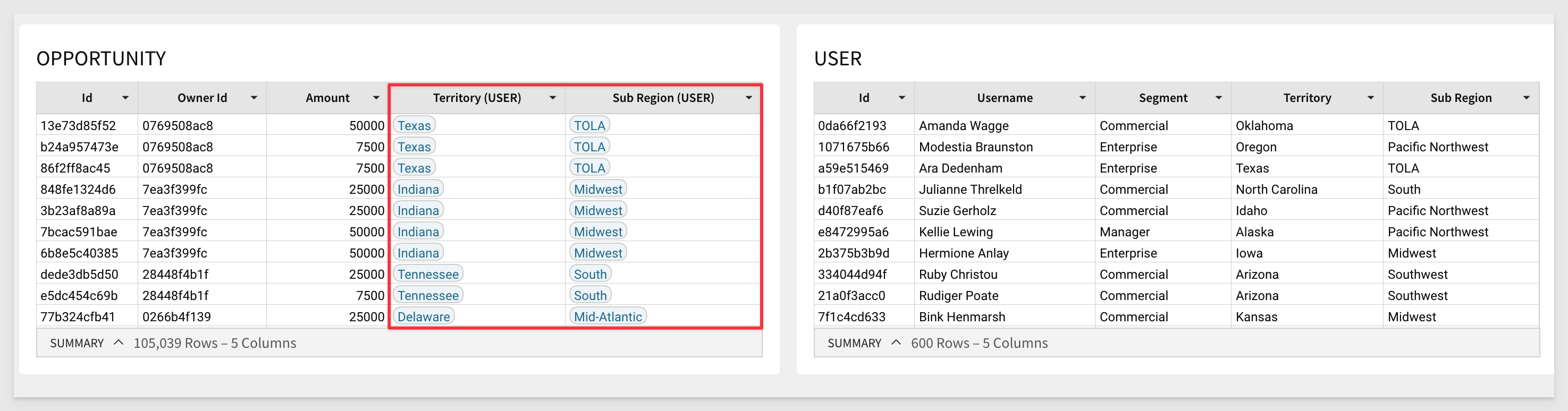
Do the same steps but this time add the USERS column SubRegion:
Your page should now look like this:
Let's add a chart that shows the current distribution of Sales by Region, so that we can evaluate what adjustments to territories may be needed.
Create a Child Element / Visualization from the Opportunity table. Configure it as follows to show the total sales by region:
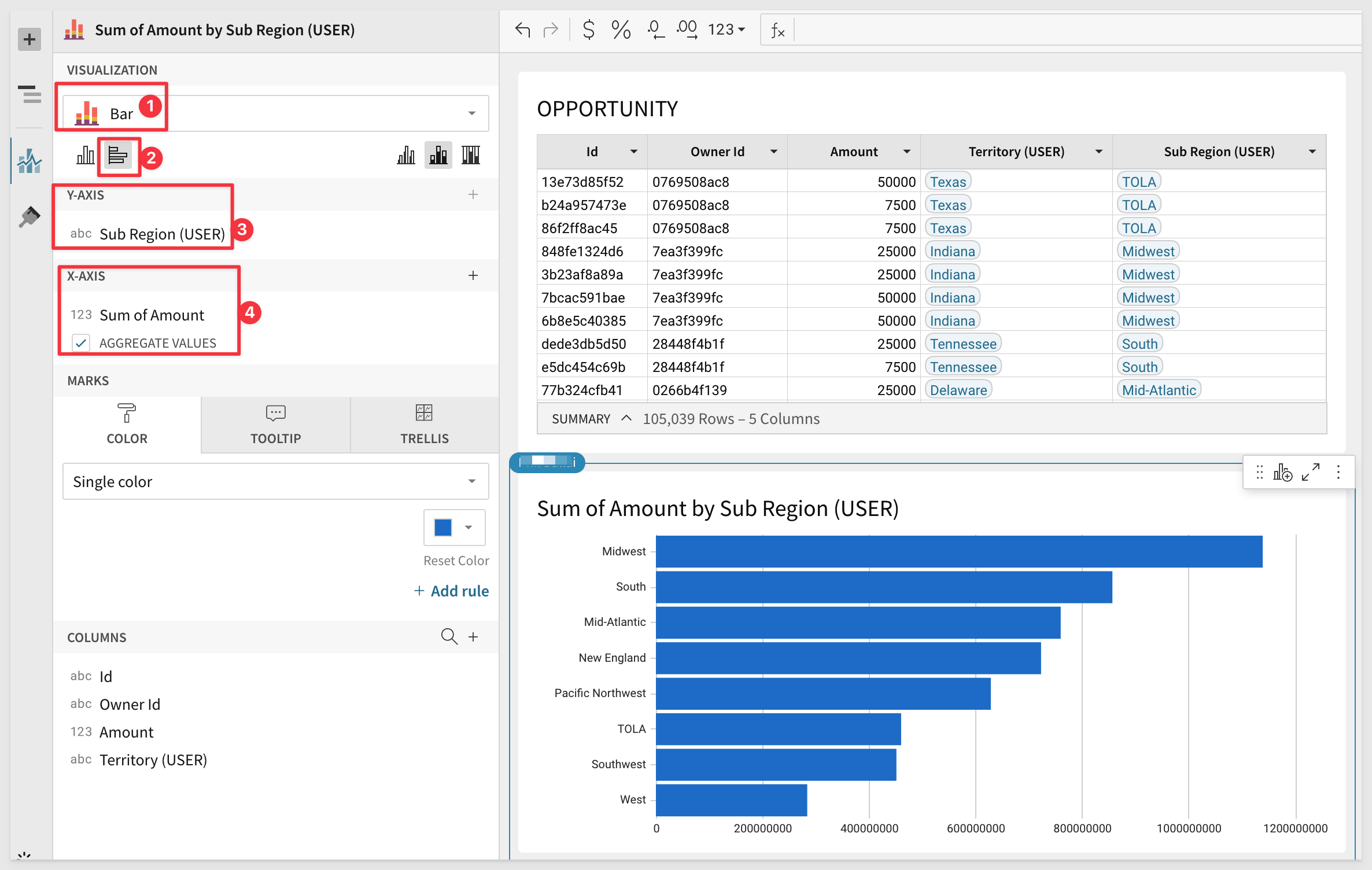
Our chart is sorted by Sum of Amount to have the largest on top. Rename the chart to Sum of Amount by New Sub Region - BEFORE
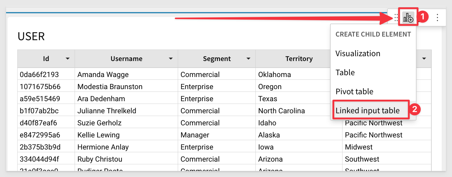
We are ready to add a method for users to reassign territories, and see the effect in real-time in terms of total regional sales.
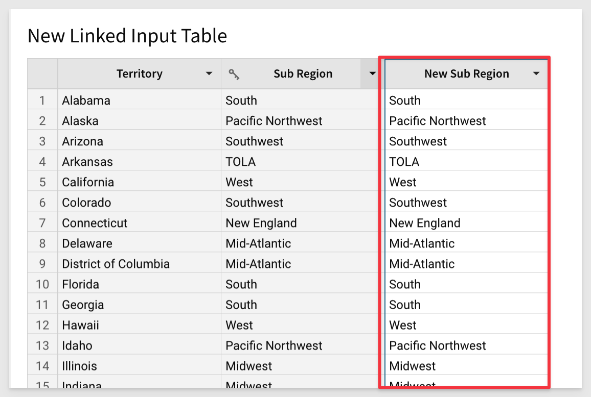
Create a new Linked input table off the USER table:
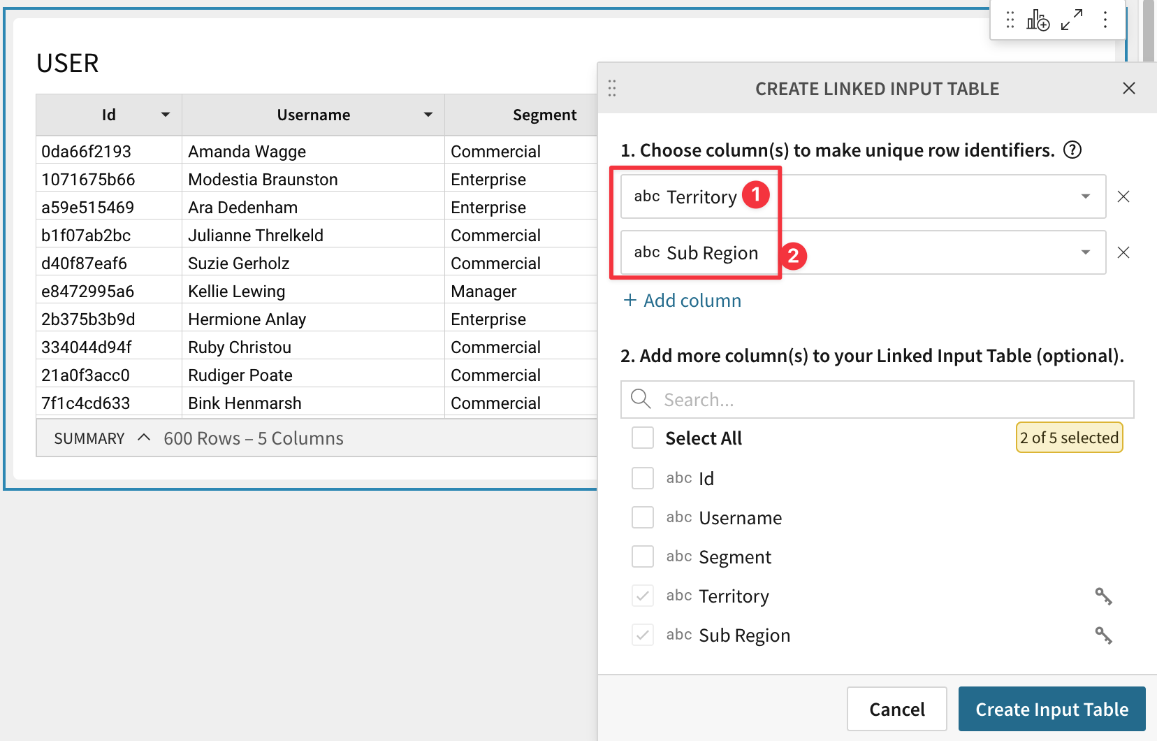
In the new Linked Table, click the Sub Region column drop and add a new Text Column:

Now copy the values from the Sub Region column (click the column and use ctl+v or command+c) and then paste into the new column (use ctl+v or command+v).
Rename the new column to New Sub Region.
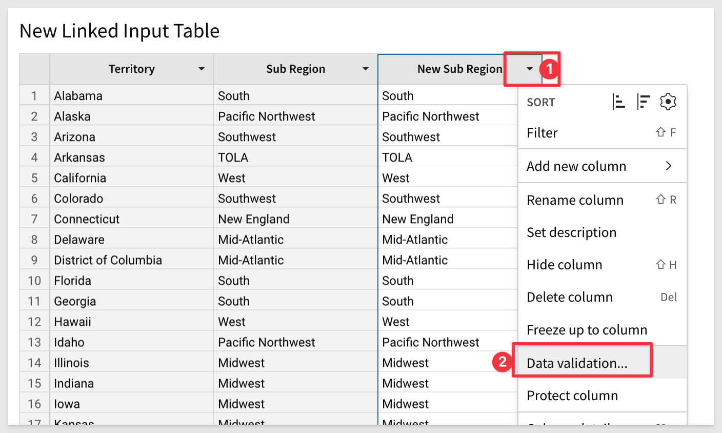
Now that we have a column where a user can change the value of region, we should add Data Validation
In the new input table, click the new column New Sub Region and select Data Validation from the list:
...and configure it as follows:
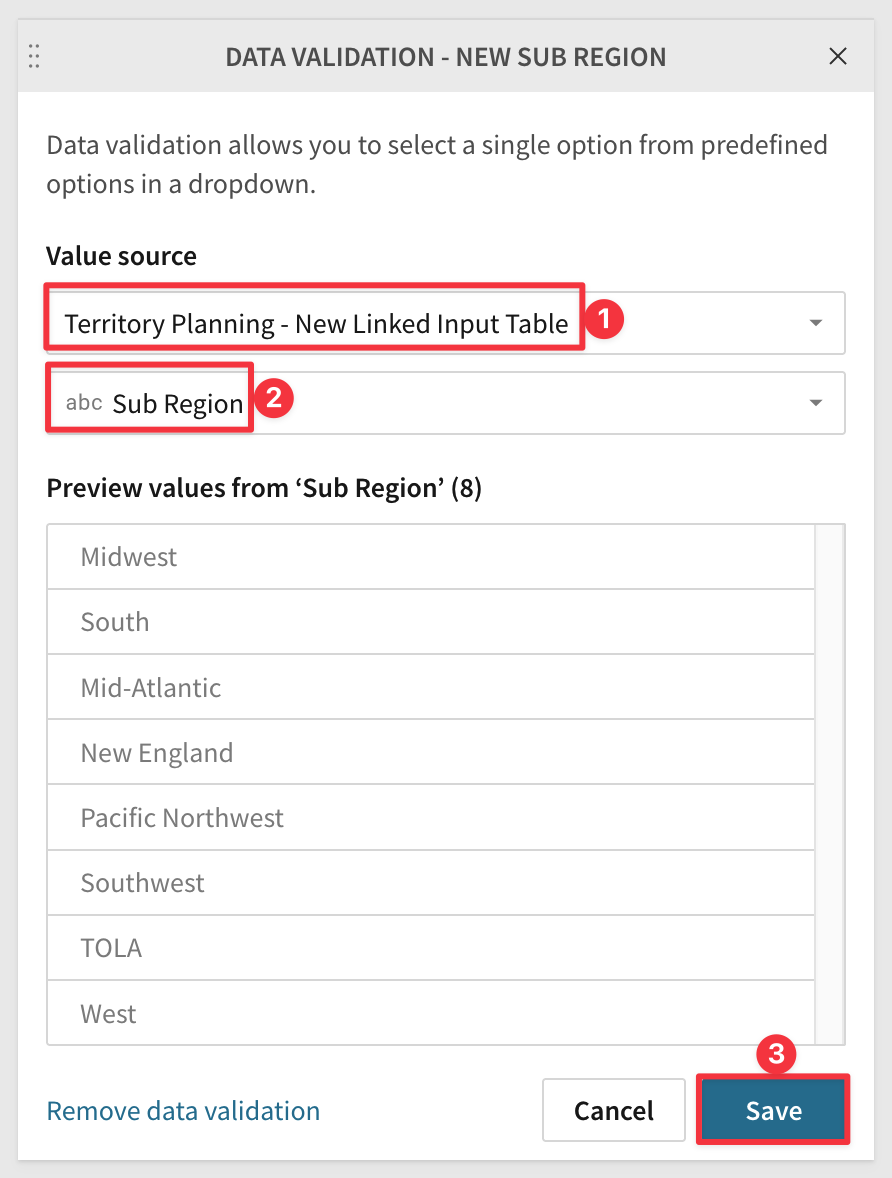
Now users are limited to selecting valid values from data that exists in USERS table.
Even though we configured the new column's data validation to point to the input table, the Sub Region column is "linked" to the data coming from the Users table, so it will always be up to date.
Next we want to add a New column via lookup to the Opportunities table.
Configure it as follows We should see 100% match (item #4):
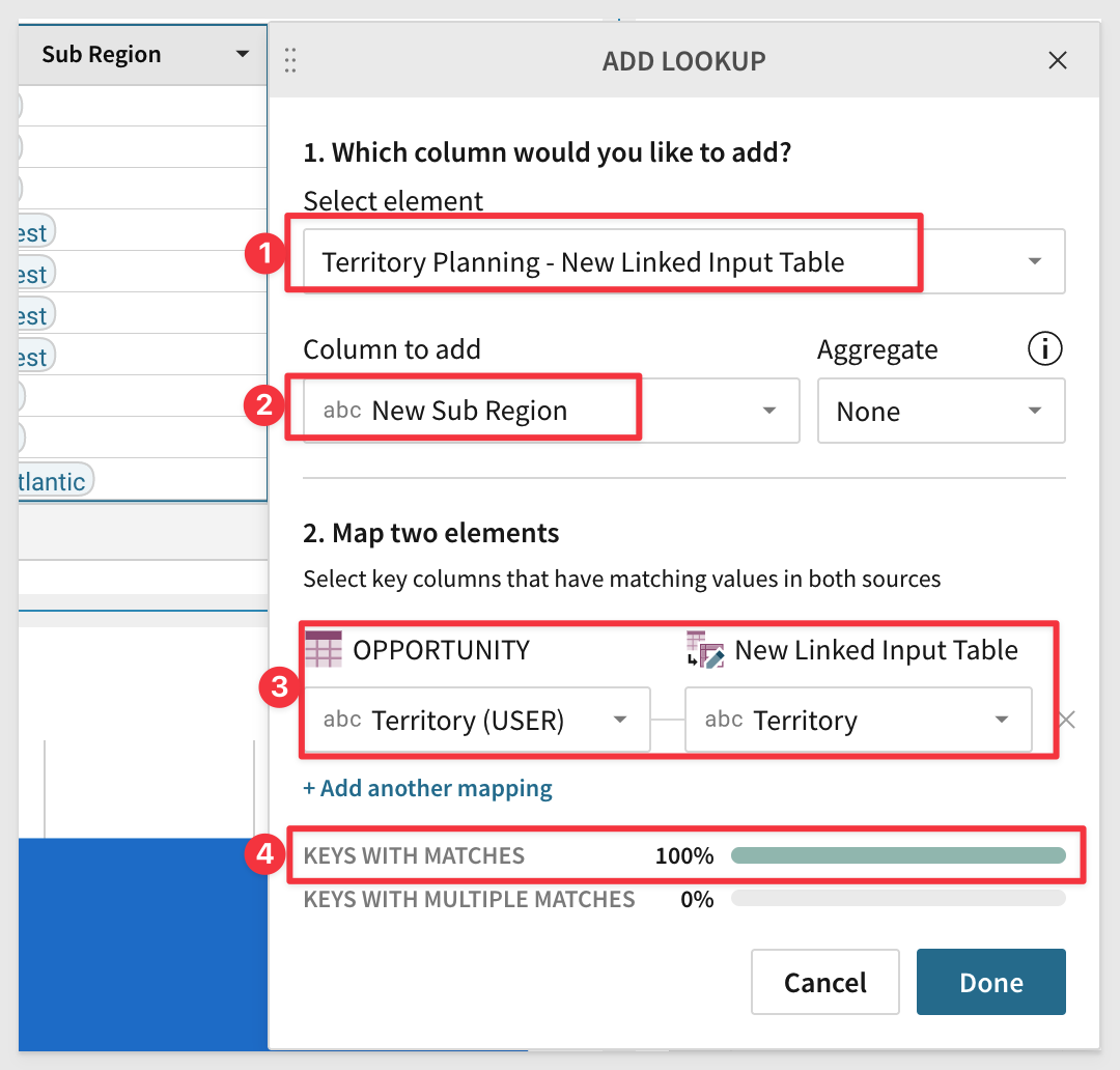
Rename the new column from New Sub Region (New Linked Input Table) to New Sub Region.
The Page now looks like this (after some re-sizing and arranging to suit your preference). Use any layout you want.
Lastly, we will add another visualization (as a child of the Opportunities table) to represent the "after" state of user changes on the linked input table.
Add a new Child Visualization and configure it as follows:
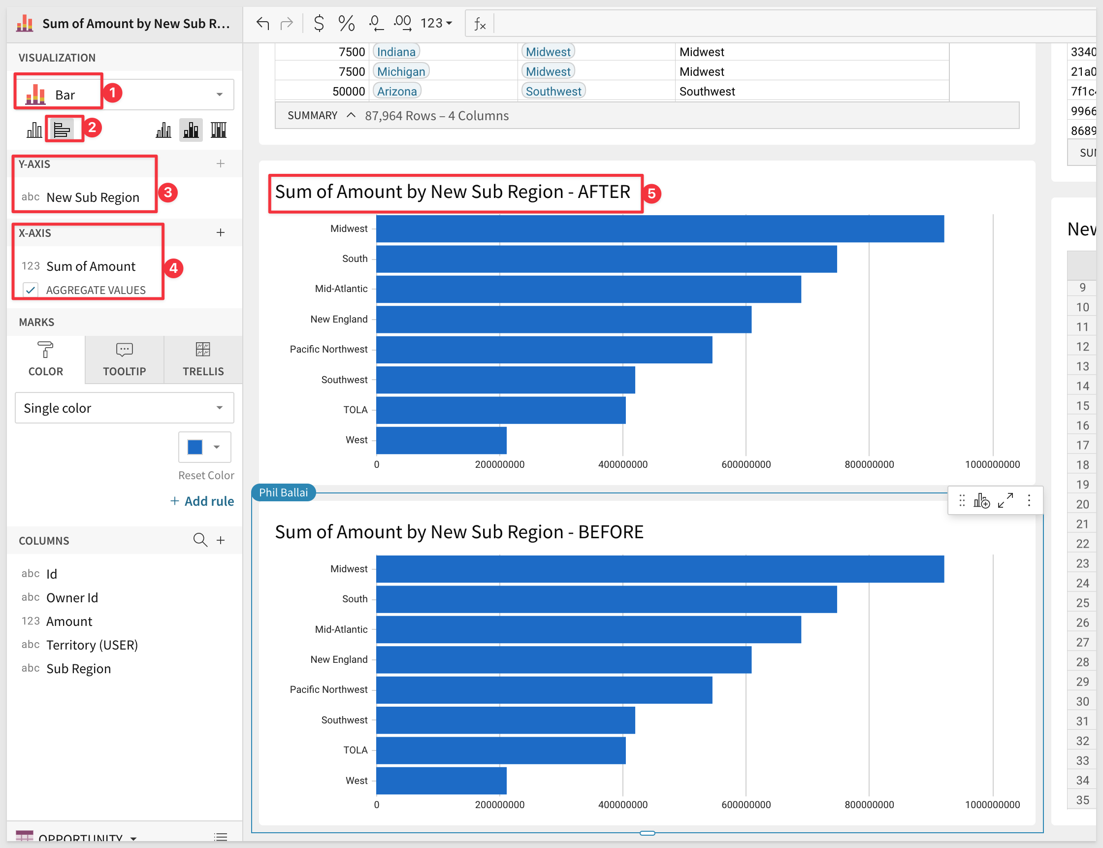
Rename the chart to Sum of Amount by New Sub Region - AFTER.
We are ready to evaluate the Territory, and make some adjustments.
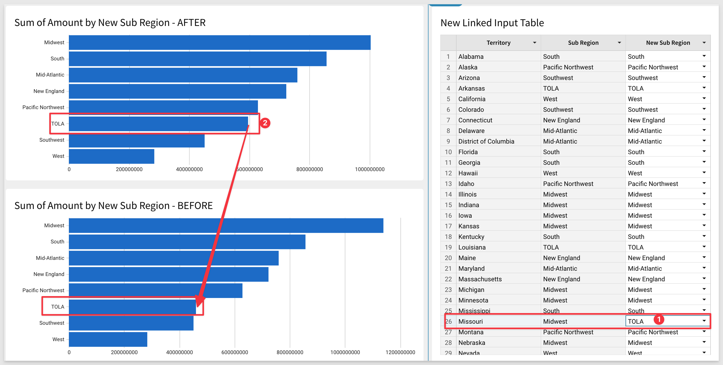
First. we need to see why the Midwest so much larger than the TOLA in terms of sales. We want to close this gap if we can.
In the Before chart, click the Midwest bar and Drill down into Territory.
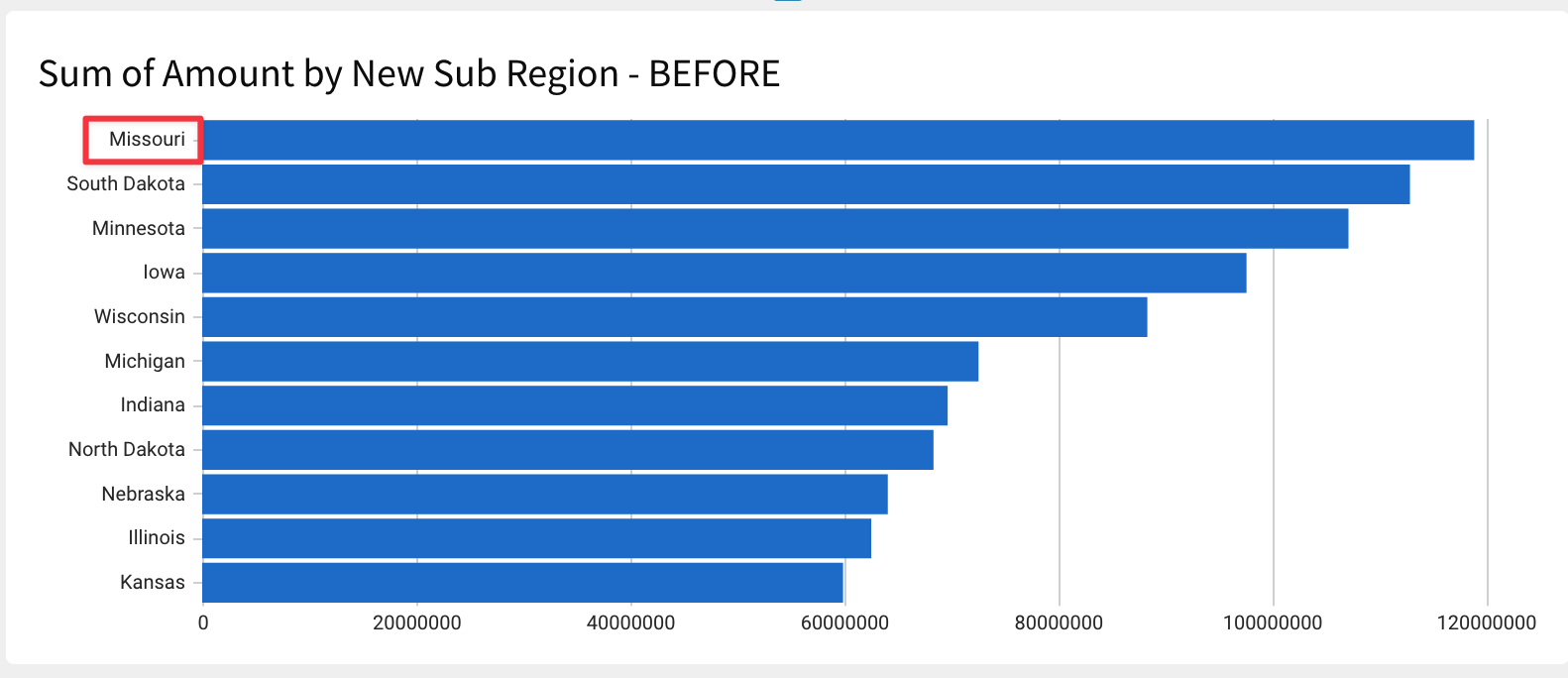
We can now see that Missouri is top of the chart. We wonder what if we reassigned it to TOLA?
Locate the Missouri in the New Linked Input Table / Territory column and change it's assignment in New Sub Region.
You can see that the AFTER chart recalcuates and TOLA is now larger with MidWest smaller but still not close enough.
Also change the New Sub Region for Iowa to be in TOLA.
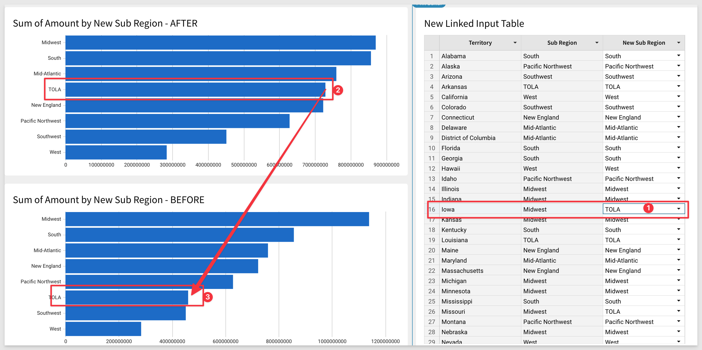
The gap is much better now, Mike is happy.
Many customers are embedding content in their internal and external business applications. Now you can also embed input tables and really take it to the next level for your users. With input tables your applications can become more than just a way to communicate TO your users. Capturing small amounts of critical data from your customers opens up that "conversation" to be two-way.
This QuickStart assumes familiarity with how to embed in Sigma.
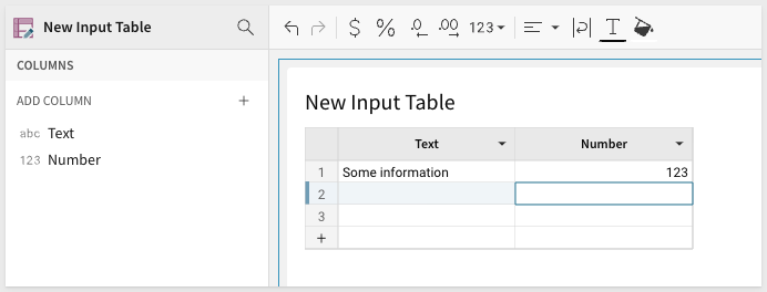
Create a new workbook and add a new empty input table table to the page. You will be prompted to provide a location to save the input table date. We will use the Sigma Sample Database.
Now add another column and set it's type to number.
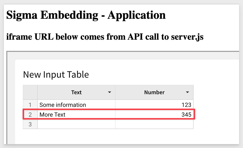
Enter a line of data and your page should now look like this:
Click the input tables menu and enable Allow data editing in explore mode.
Publish the workbook.
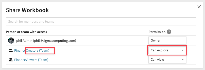
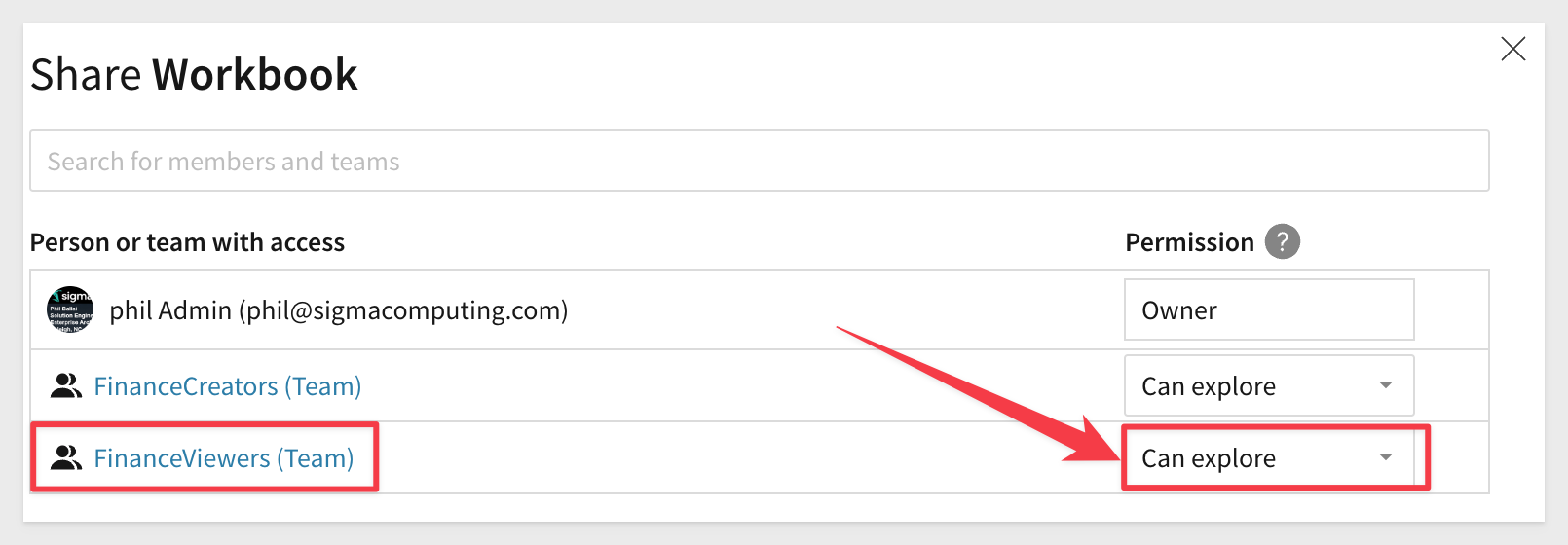
Make sure that the workbook is Shared to the Creator team with Explore or Creator rights:
Using the methods outlined in the Quickstart Embedding 3: Application Embedding, configure this workbook page into an embed.
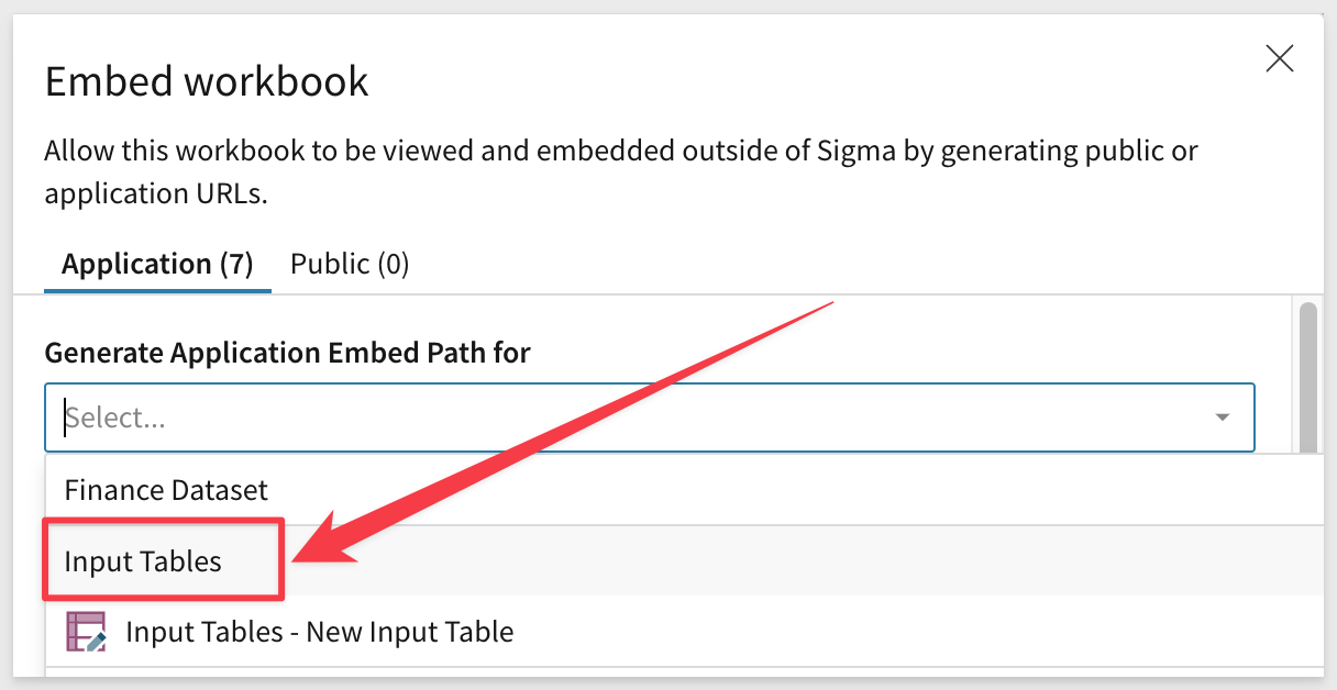
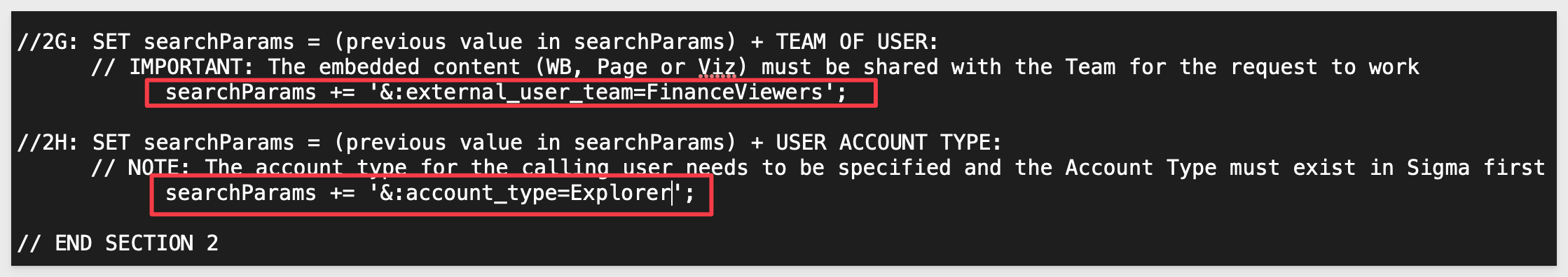
We will need to adjust server.js for the Embed Path, User Team and Account Type:
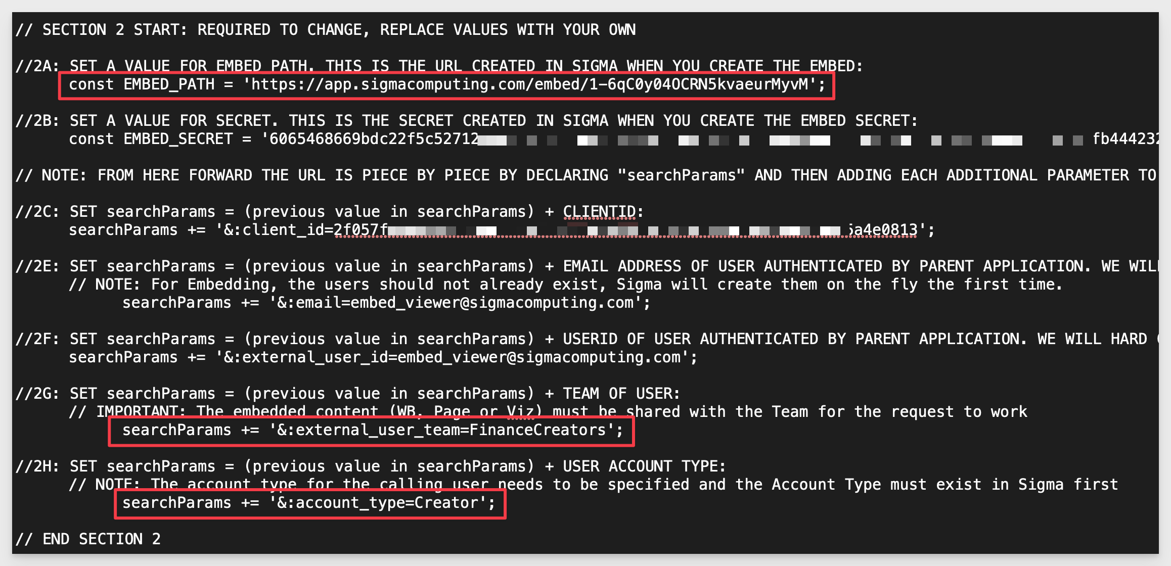
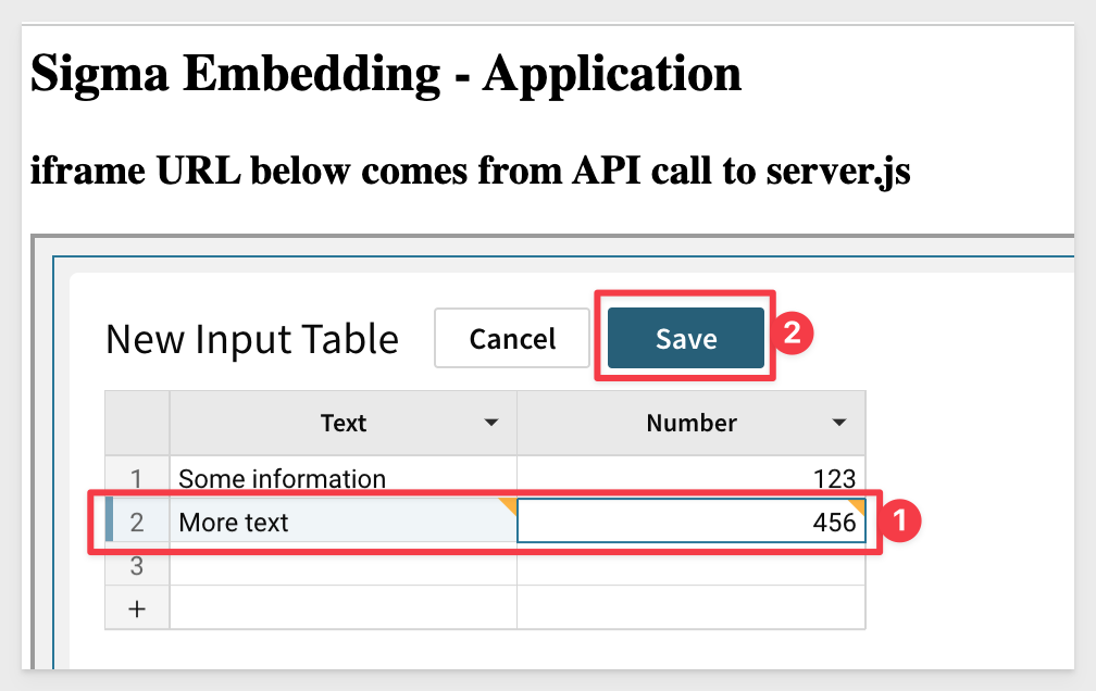
Assuming you started Terminal and ran supervisor server.js without error, browser to http://localhost:3000. You should see your embedded input table.
Enter some text and click Save.
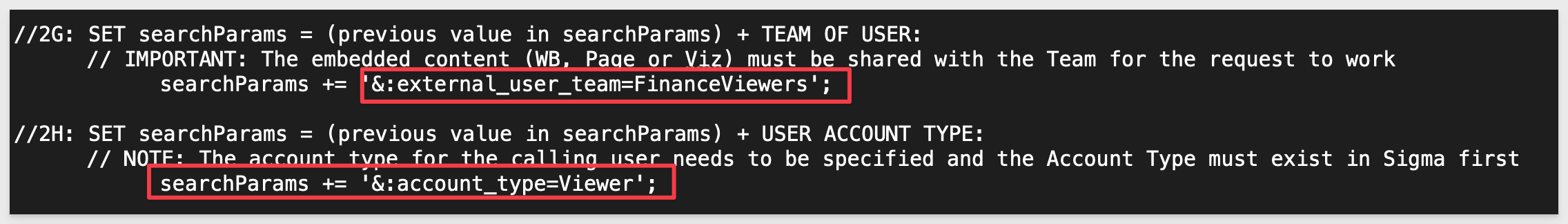
Adjust server.js for the User Team and Account Type to lower the access to Viewer:
Refresh the browser and see that the information is as we entered it but there is no Edit functionality for this Viewer user.
If you recall, we enabled Allow data editing in explore mode. Lets test that.
In the workbook / Sharing change the Viewer to use the Explore role:
Update server.js for account_type and external_user_team and save the file:
Refresh the browser and see that we have the Edit button.
There are times when capturing a small amount of data from a Sigma user can be very valuable to the business. This presents some challenges:
- Will you have to build some new application to capture the data?
- When is the right time to capture the data?
- Will the users accept another tool?
- Once we have the data, how will it relate to existing warehouse data?
- Lots of other questions to be sure!
Since users are already using Sigma (or spreadsheets and should be using Sigma instead!), input tables can help solve this problem. Why not just create a Sigma workbook and augment it with the ability for the user to enter small amounts of data in real time? Sigma will do the heavy lifting of UI and data operations to store the data in your warehouse.
Allowing users to add/supplement warehouse data opens a world of possibilities. We can demonstrate how this can be done we will use a very simple example.
There is a need for accounting to update the status of Invoices, adding comments/notes but don't want to give the data entry clerk access to the accounting system.
We solution this in Sigma using input tables without involving developers or database administrators valuable time.
In our workbook, create a new Page and rename it to Data Collection.
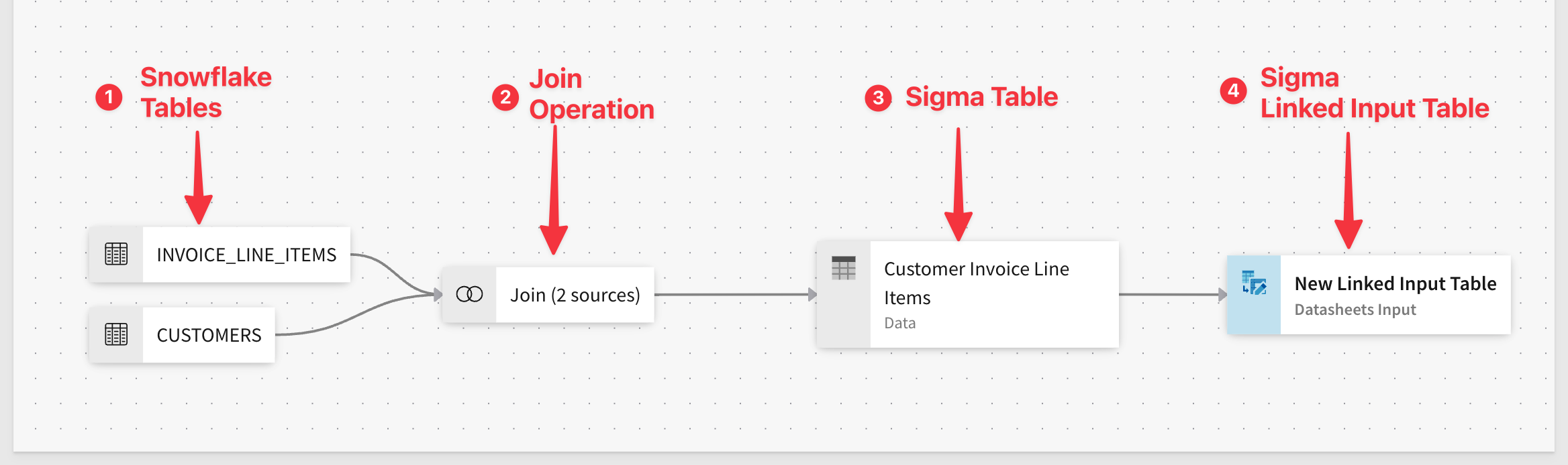
We need to use different data for this use case, joining two tables.
In our use case, the final lineage for the source data table looks like this:
In Edit mode, navigate to the Data page.
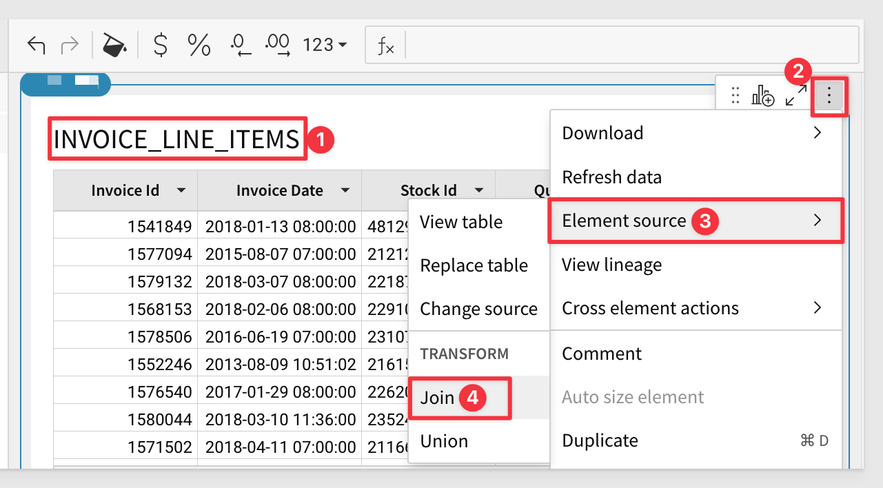
Add a new table for INVOICE_LINE_ITEMS as shown:
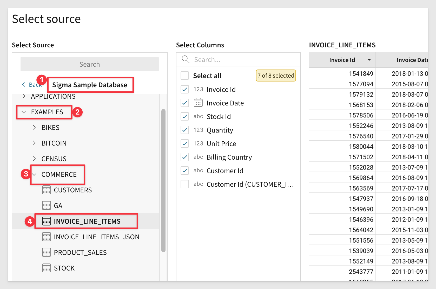
Join the CUSTOMERS table to this INVOICE_LINE_ITEMS as shown:
Configure the Join as follows:
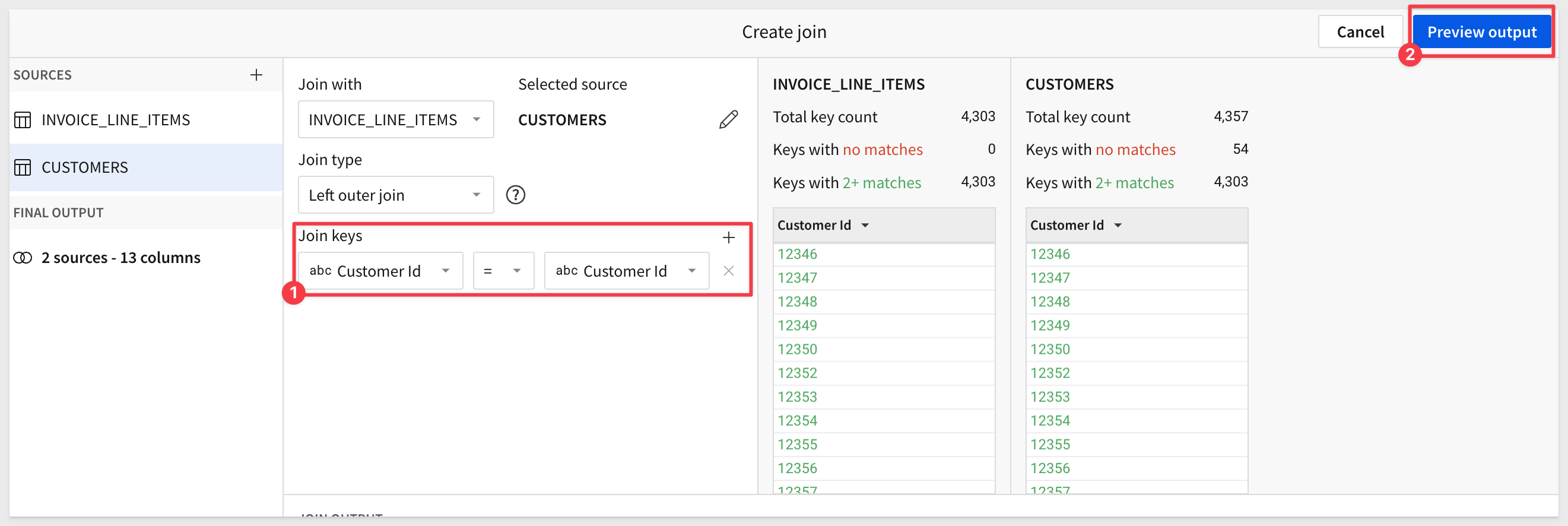
After clicking Preview to look at the result set, click Done:
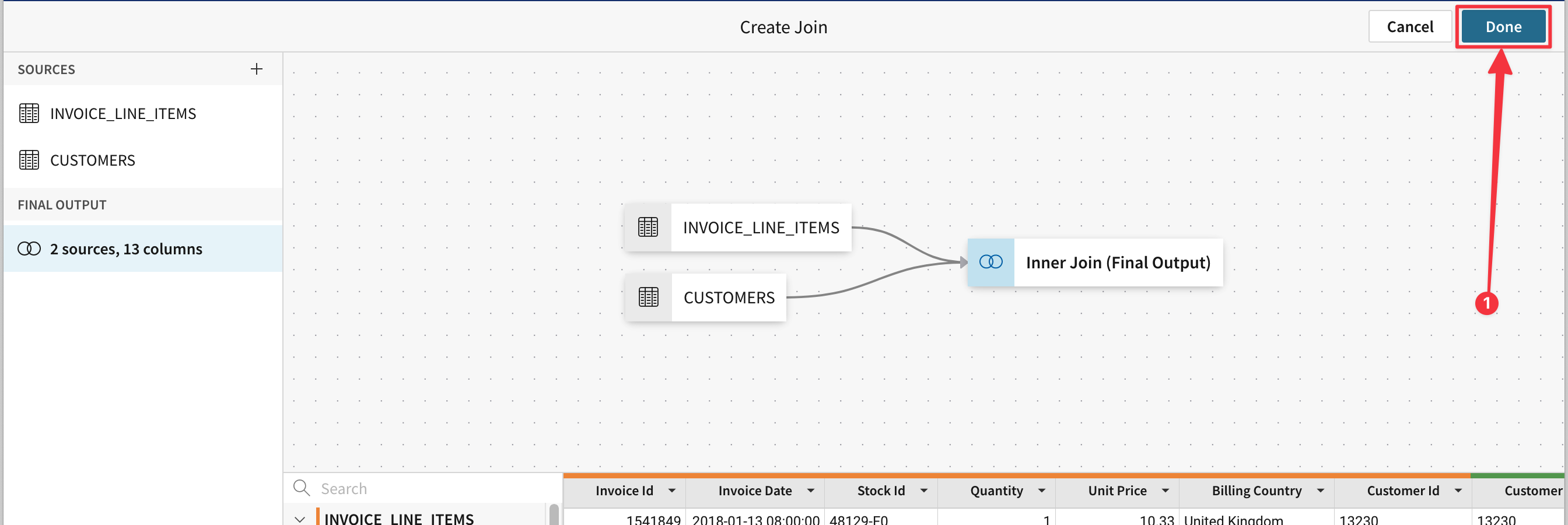
We don't need every column so let's delete the ones we wont require:
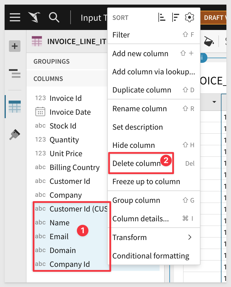
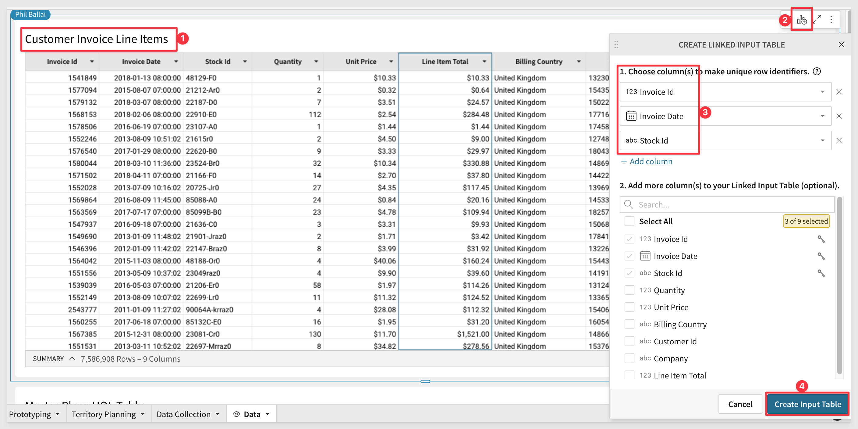
Rename the new table to Customer Invoice Line Items.
Now create a Linked Input Table, selecting the columns as shown:
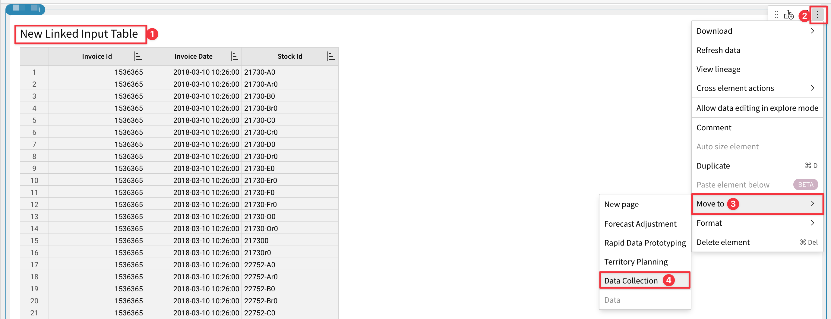
Move the new input table to the page Data Collection:
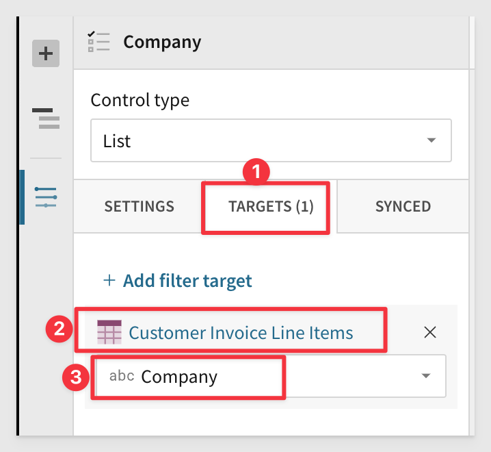
We want the user to be able to filter the input table to specific Companies.
Add a new Element / Control Element / List Value element and configure it as follows:
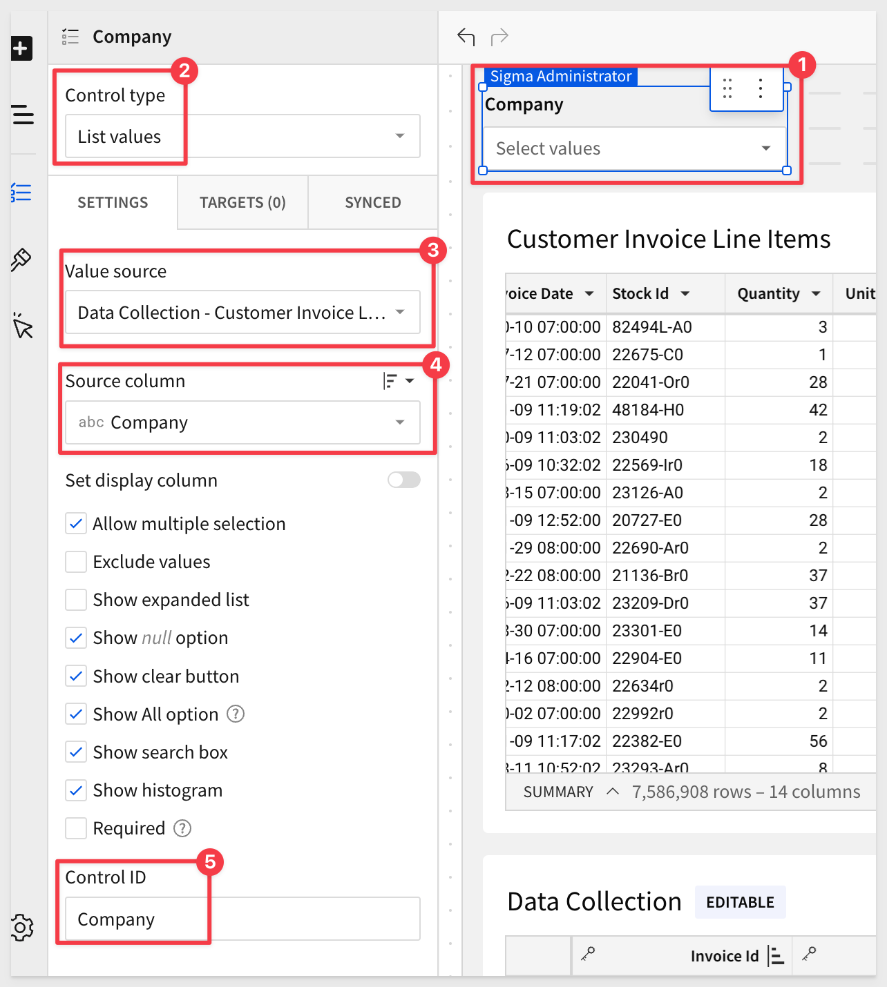
Set the Target as:
We now are ready to add our columns that are enabled for data capture.
Add a new Column to the input table called Status.
Add another new Column to the input table called Notes.
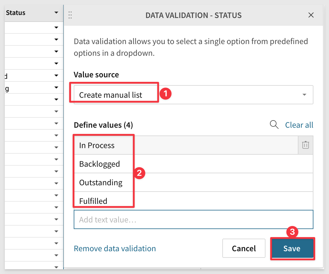
We demonstrated data validation in an earlier use case, but this time will just limit the Status column to values we will manually provide:
Now we can filter by Company, select a Status and add Notes.
The last step before we test, is to set the data entry permission:
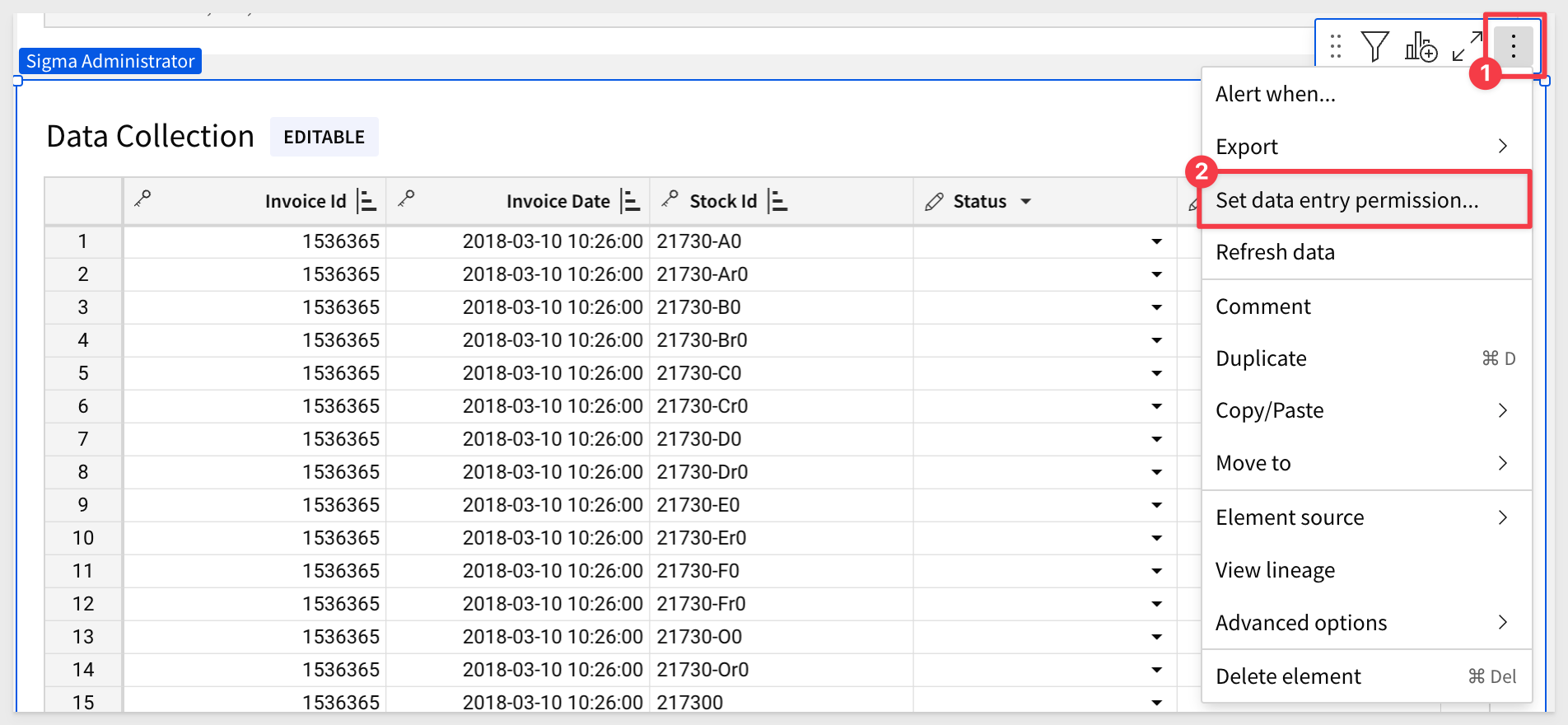
Sigma presents two choices explaining who can edit the input table:
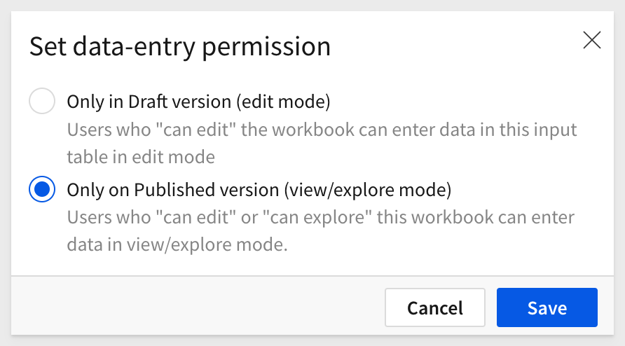
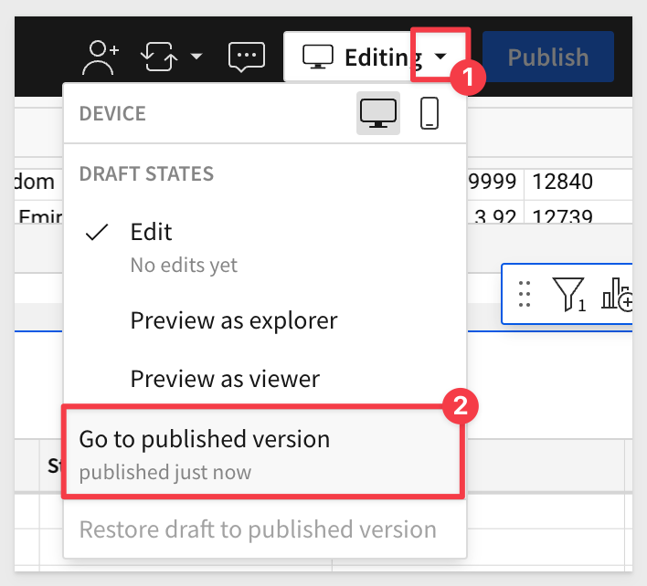
Select Only on Published version (view/explore mode) and click Save.
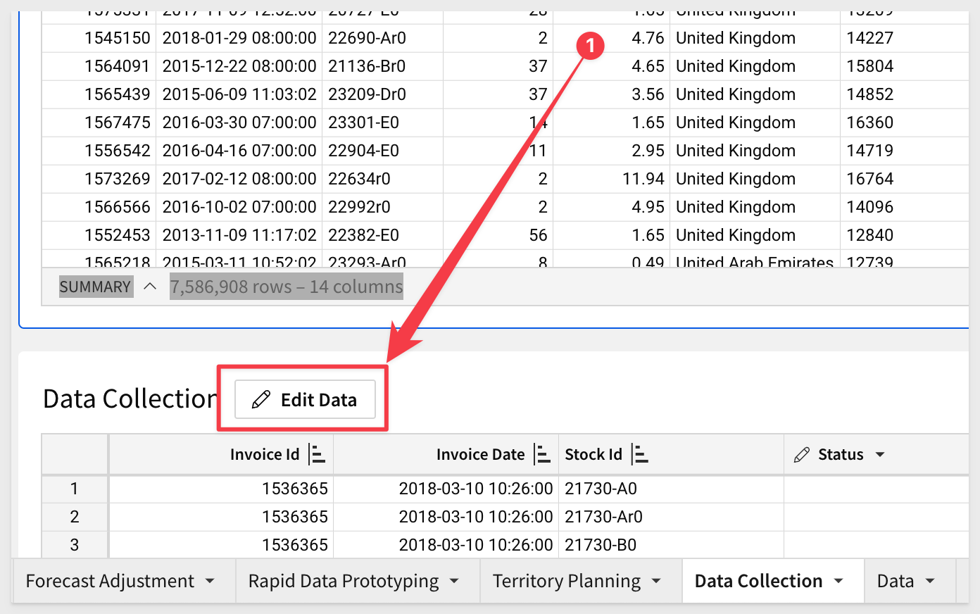
Publish the workbook and go to the published version, so that we are looking at this as the end-user would see and work with it.
Now we have an Edit Data button. Click that:
Lets test by updating the first four records as shown for each Status:
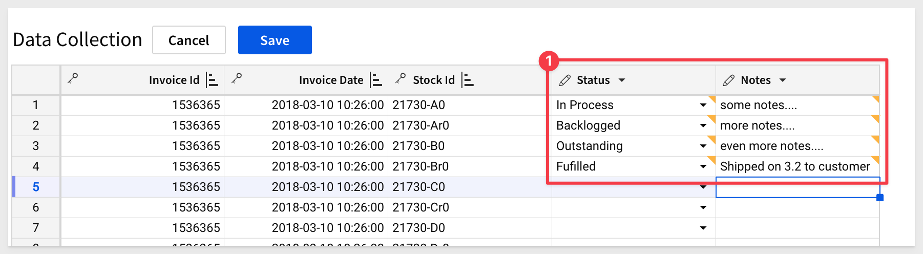
Click the Save button.
In this QuickStart we covered three popular used cases for Sigma input tables in great detail.
Additional Resource Links
Be sure to check out all the latest developments at Sigma's First Friday Feature page!
Help Center Home
Sigma Community
Sigma Blog