Houston, We Solved the Consumption Estimate Problem: A Hands-On Lab with Sigma's New Activity Sizing Application (NASA)
Welcome to NASA, Sigma's New Activity Sizing Application! In this hands-on-lab you will be taking on the role of a Snowflake Sales Engineer.
Your mission:
Provide a detailed readout of POV activity and a data-backed prediction of future usage as your customer, Papercrane Inc., prepares to sign their Cap 2 Deal with Snowflake.
In this hands-on lab, you will take on the role of a Snowflake Sales Engineer.
Background:
Papercrane recently completed a two-week POV with Sigma and hopes to understand how onboarding this new workload could impact their overall Snowflake credit consumption.
As you work together to scope their new Snowflake contract, you will leverage the Sigma platform—and the Sigma partnership—to analyze usage data, identify trends, and build a consumption estimate, culminating in a POV readout for Papercrane Inc.
Target Audience
Participants of Snowflake SKO 2025 who are interested in getting some hands-on with Sigma.
No SQL or technical data skills are required for this hands-on-lab.
Prerequisites
- A computer with a current browser. It does not matter which browser you want to use.
- Access to a Sigma environment, using the Sigma tile in Okta.
- A Snowflake demo environment.

2.1: Find "Sigma - New Activity Sizing Application" in DataOpps.Live and follow the Set up new solution steps to deploy the data and workbook.
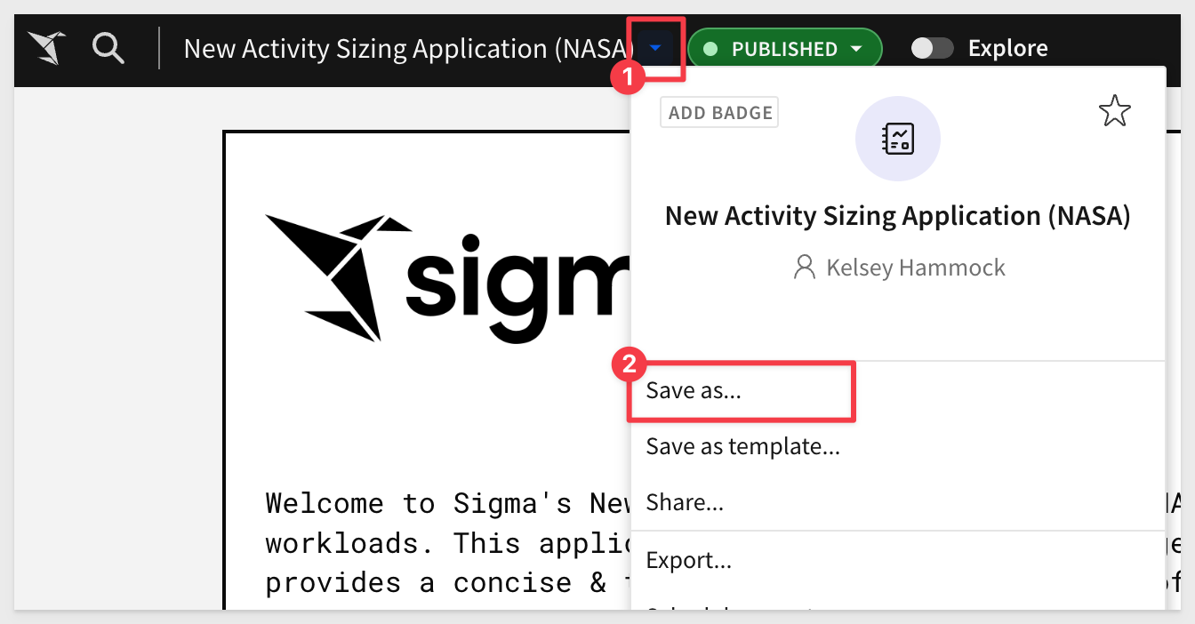
3.1 Once the workbook is open, click the  by the template title and select
Save As.:
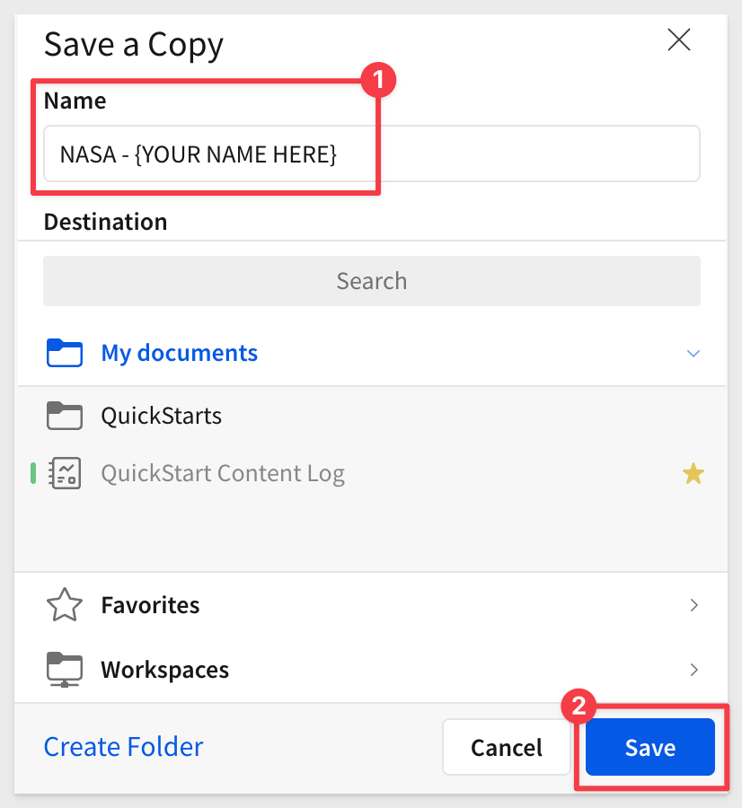
3.2 Rename the workbook NASA - {YOUR NAME HERE} and click Save.:
We also need to download a zip file that contains two CSV files and one text file of a POV readout via Gong.
We will use these later in the lab.
Extract these somewhere on your local computer where you can find them later.
4.1. Using the buttons on the home page, navigate to the Analysis tab:
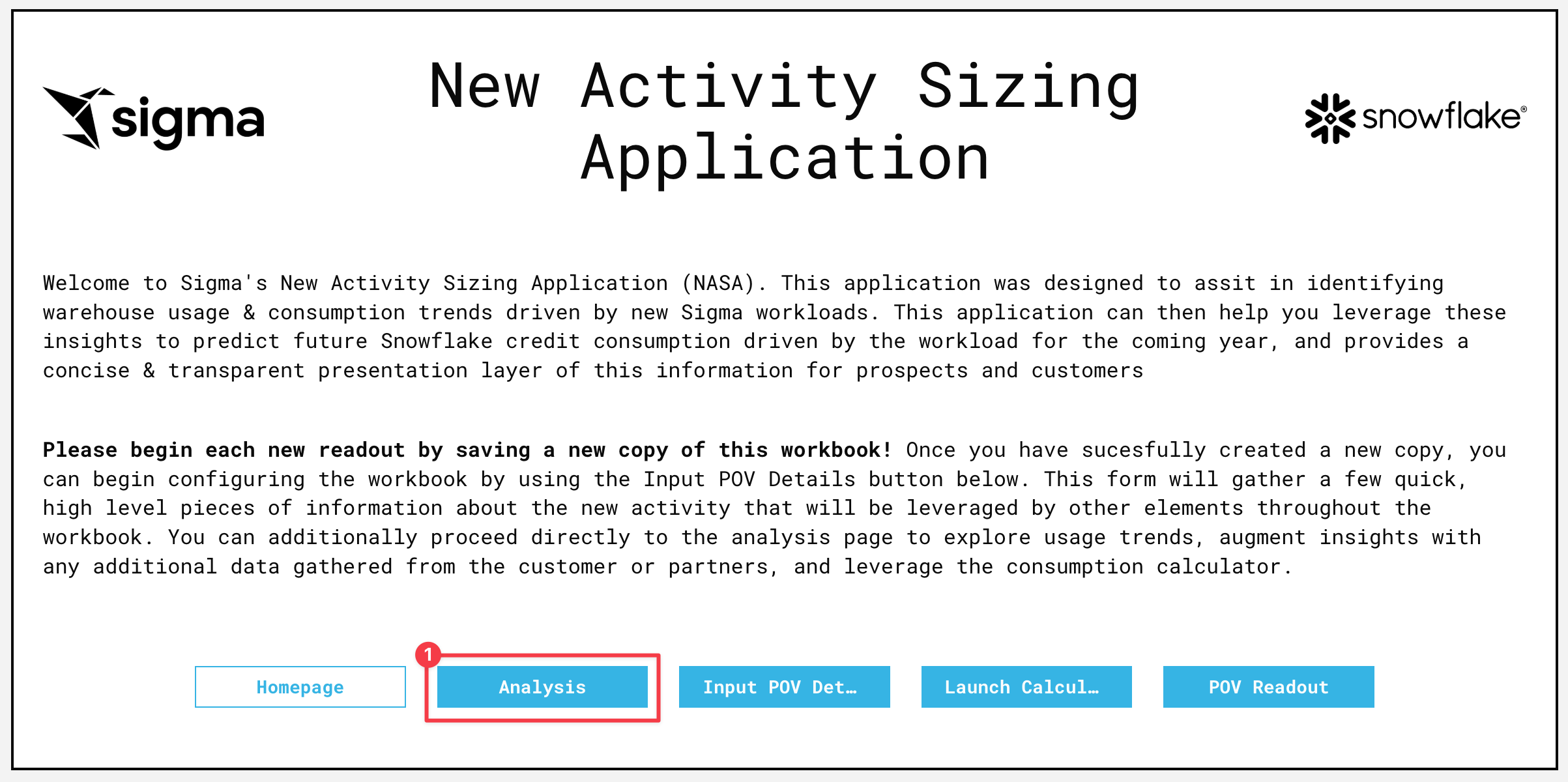
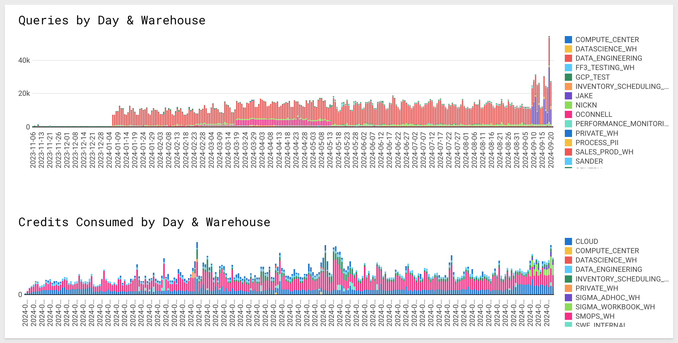
On this tab, you should see the Snowflake query history and warehouse metering tables, as well as high level visualizations of the number of queries run by each warehouse and credits consumed.
4.2 You will notice the trend in usage has increased in the last two weeks as the result of your customer's active POV with Sigma, and that two warehouses seem to be driving this trend: SIGMA_ADHOC_WH and SIGMA_WORKBOOK_WH:
Let's narrow this data down to just the new workload.
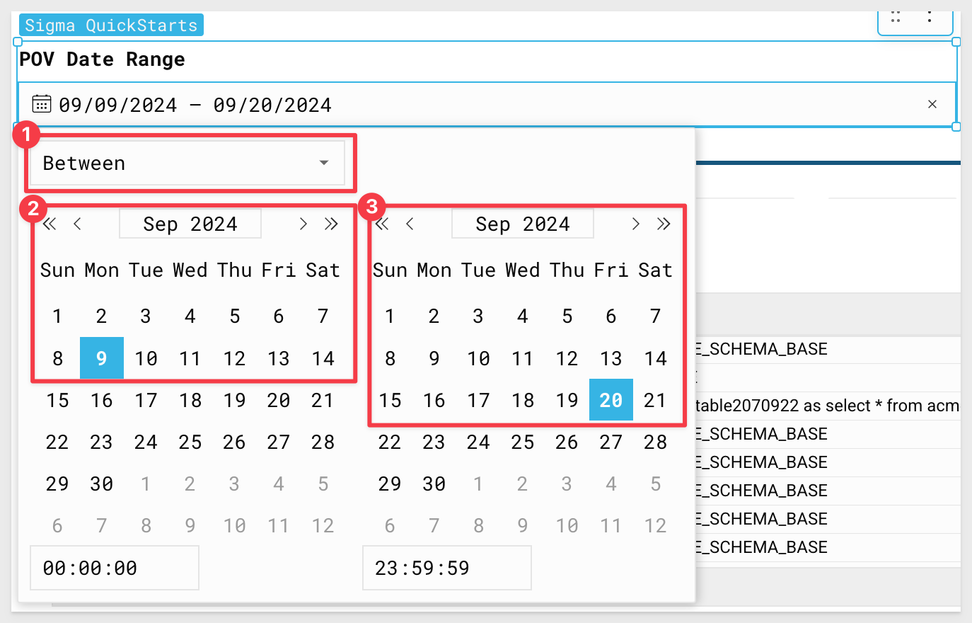
4.3 Using the Select POV Date Range filter, select the dates 9/9/24 - 9/20/2024:
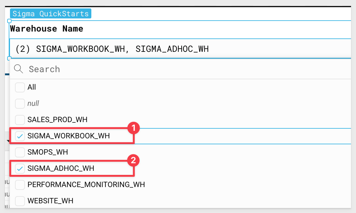
4.4 Using the Warehouse Name Filter, select SIGMA_ADHOC_WH and SIGMA_WORKBOOK_WH from the drop down.
We can now see usage data related only to the new workload the customer is trying to scope.
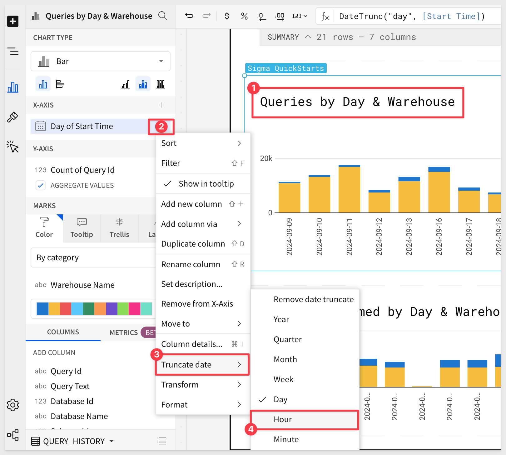
4.5 Click on the Queries by Day & Warehouse bar chart. Under X-Axis you will see Day of Start Time.
Click the down arrow to the right of Day of Start Time and select Truncate Date > Hour to get a sense of the usage trends throughout the day:
4.6 Let's adjust the scale of the X-Axis to be more reflective of timeline.
Click the Paintbrush on the lefthand side, then select X-Axis.
Under Scale type, select Time:
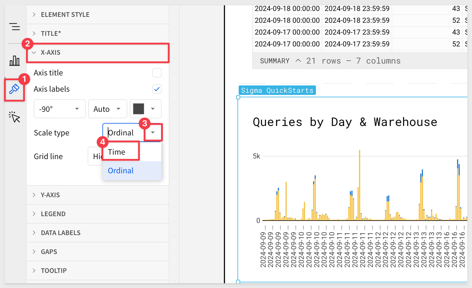
This view can help us see the way warehouse usage peaks throughout the day, with a large number of queries being fired by the new Sigma workload during peak usage times:
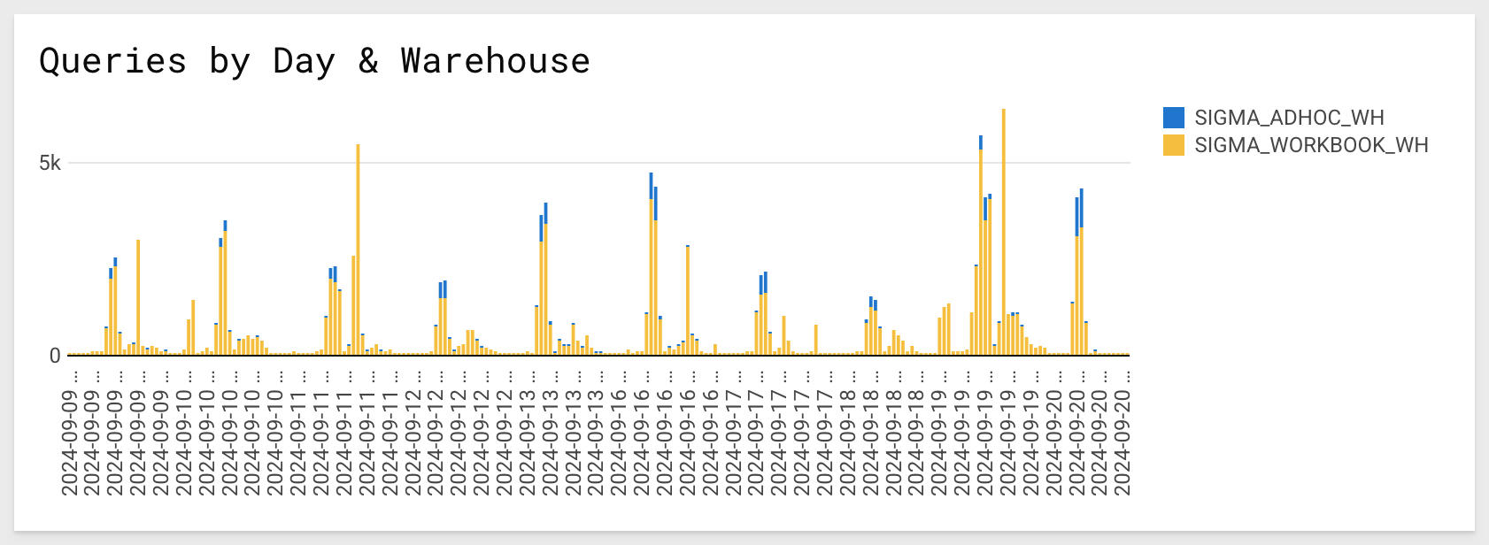
4.7 One of the more complicated aspects of a consumption estimate is trying to determine how the number of users translates to actual warehouse usage.
Luckily, our partners at Sigma have provided us Sigma telemetry and user data from the POV that we can add into our analysis.
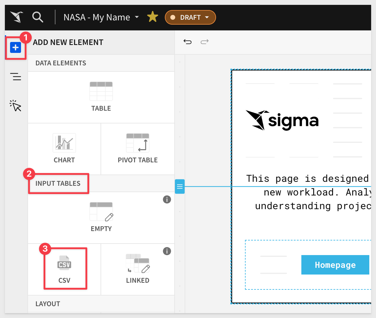
In the top left click the large plus sign to add a new element, then select CSV:
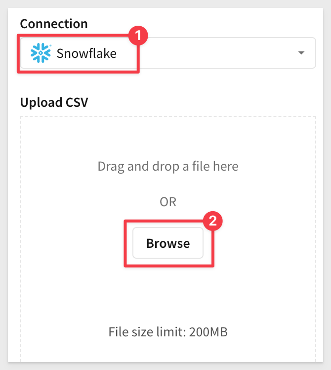
4.8 Select your Snowflake connection. Then browse for the file called UI_EVENTS.CSV or drag it and drop it to upload:
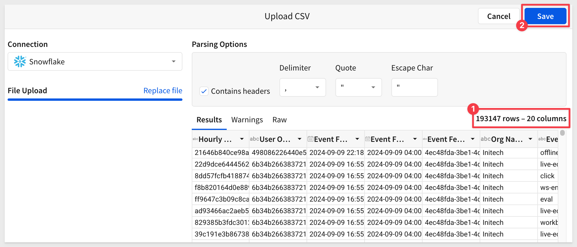
The CSV contains 192,147 rows and 20 columns. Click Save in the top right corner:
4.9 Double click the header for your new input table and rename it Sigma UI Events:
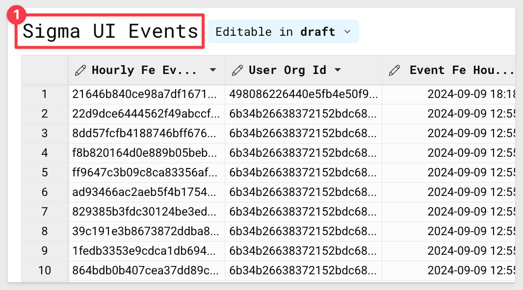
4.10 Once again, click the + sign in the top left corner, select CSV > your connection, this time uploading the file Users.CSV, and clicking Save in the top right corner when the upload is ready:
4.11 Double click the header of this new table and rename it Sigma User Information.
We now have two tables displaying information on Sigma usage, including the number of users who participated in the POC and their associated license types.
This information will help us extrapolate potential warehouse usage once the larger team onboards to Sigma and transitions into production:
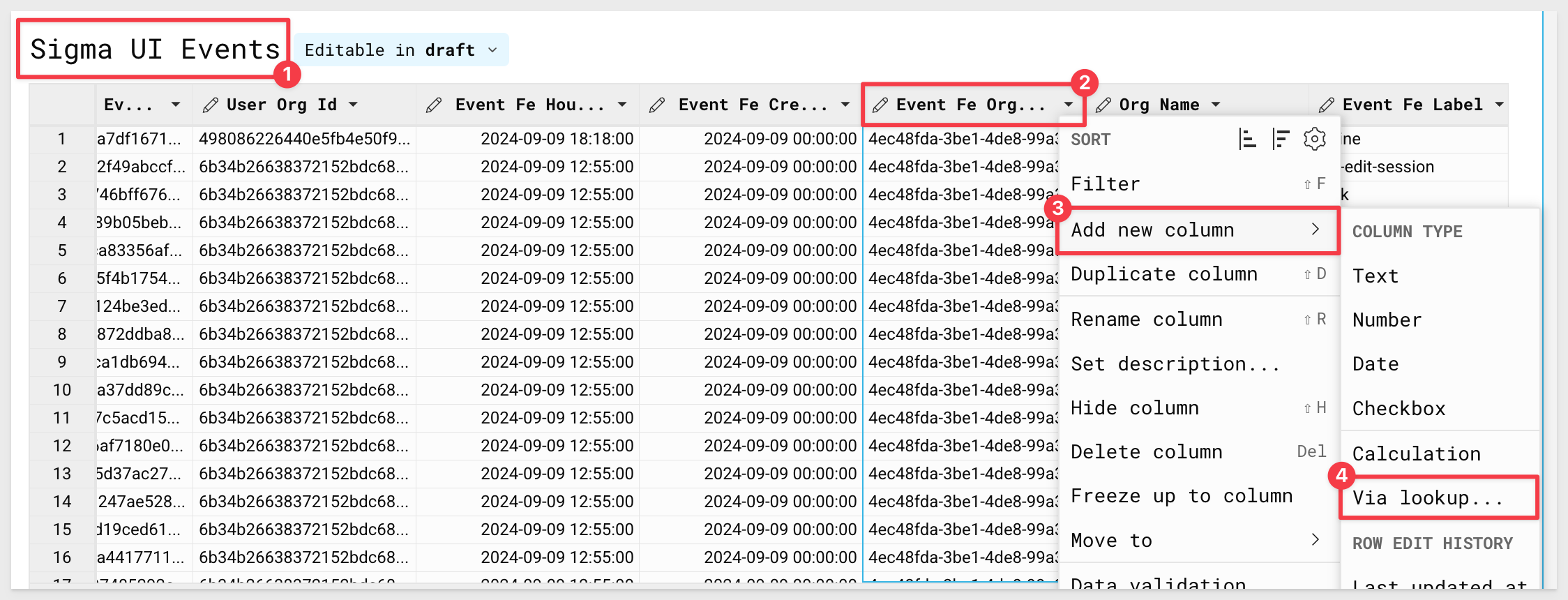
4.12 On the Sigma UI Events table, scroll through the columns until you find a column called Event Fe User Uuid.
Select the drop down next to this column, and select Add new column > via Lookup:
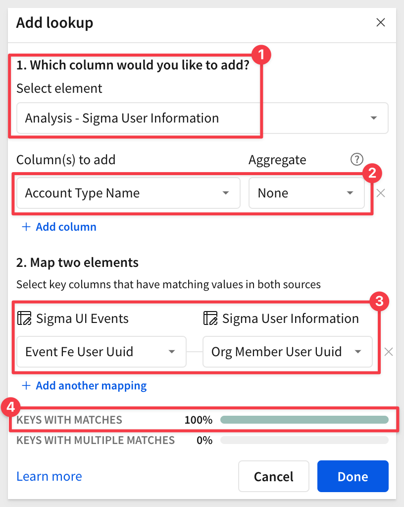
4.13 For Source, select the Sigma User Information table.
Under columns to add, select Account Type Name.
Finally, map the two elements on Event Fe User Uuid = "Org Member User Uuid.
Click the blue Done button in the bottom right.
We can now see the Sigma license type each associated event was run by:
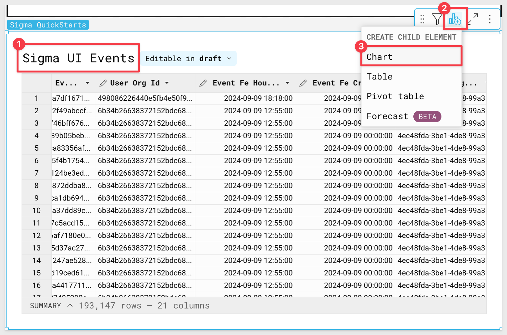
4.14 Hover over the upper righthand side of the Sigma UI Events Table object, and select Create a Child Element > Chart:
4.15 Drag Event Fe Hour UTC to the X-Axis.
Sigma automatically aggregates this timestamp at the day level.
Click the drop down to the right of this column name and select Truncate Date > Hour:
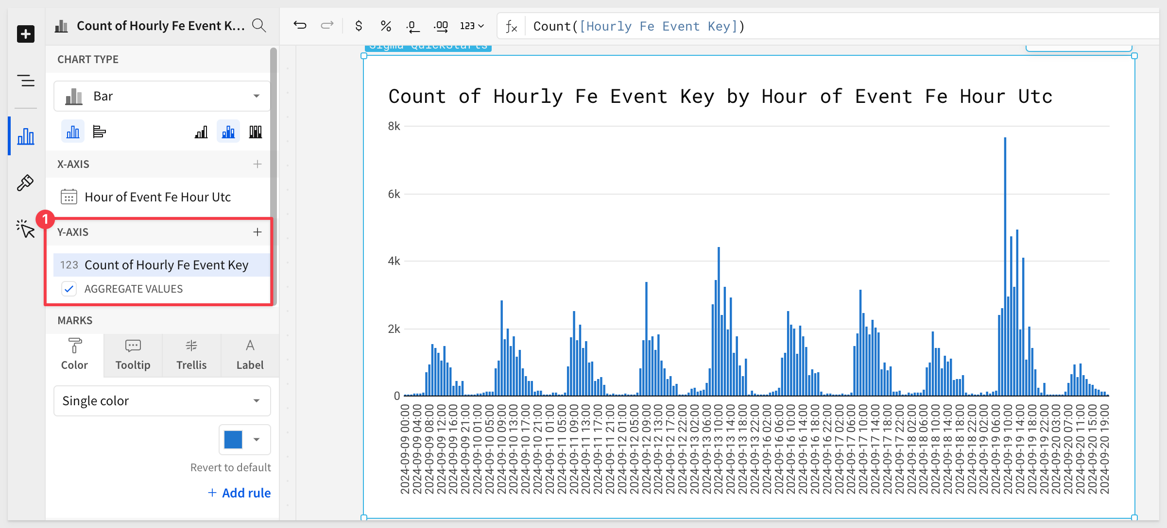
4.16 Drag Hourly Fe Event Key to Y-Axis.
Sigma will automatically make this a count of events by hour:
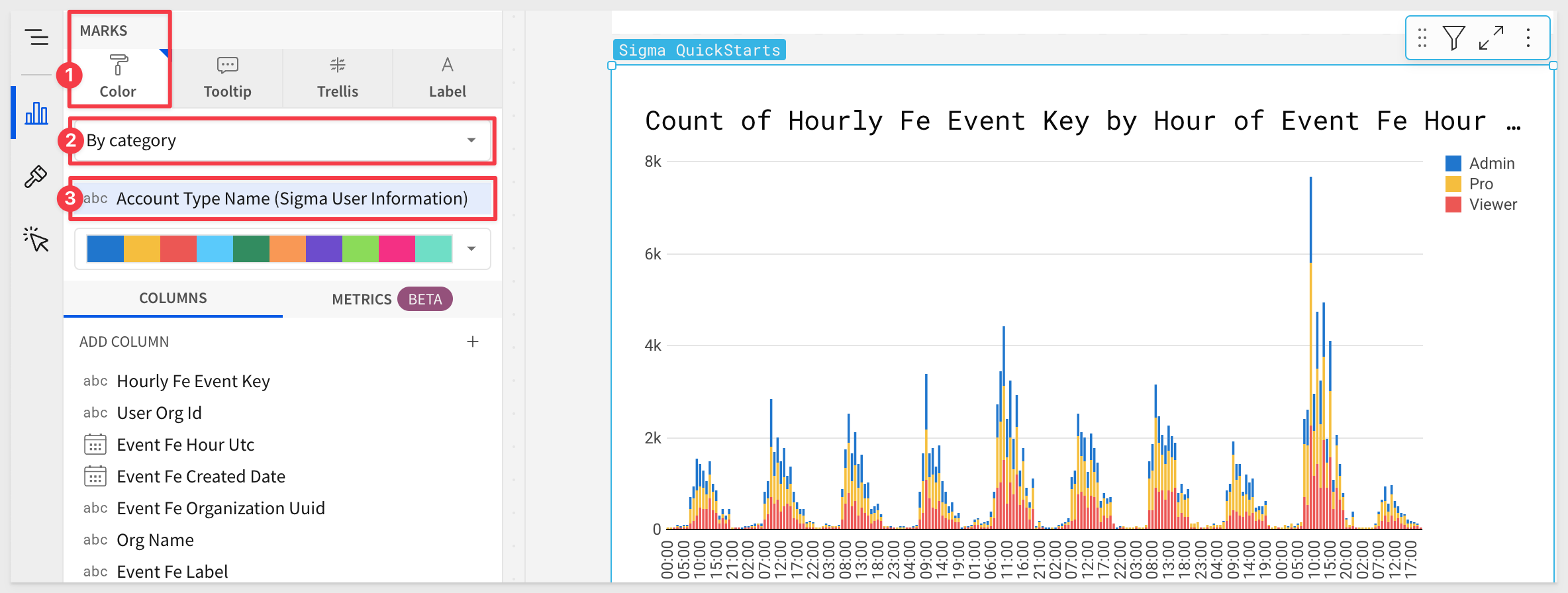
4.17 Next, change the drop list under Color and drag the Account Type Name (Sigma User Information) to the category grouping:
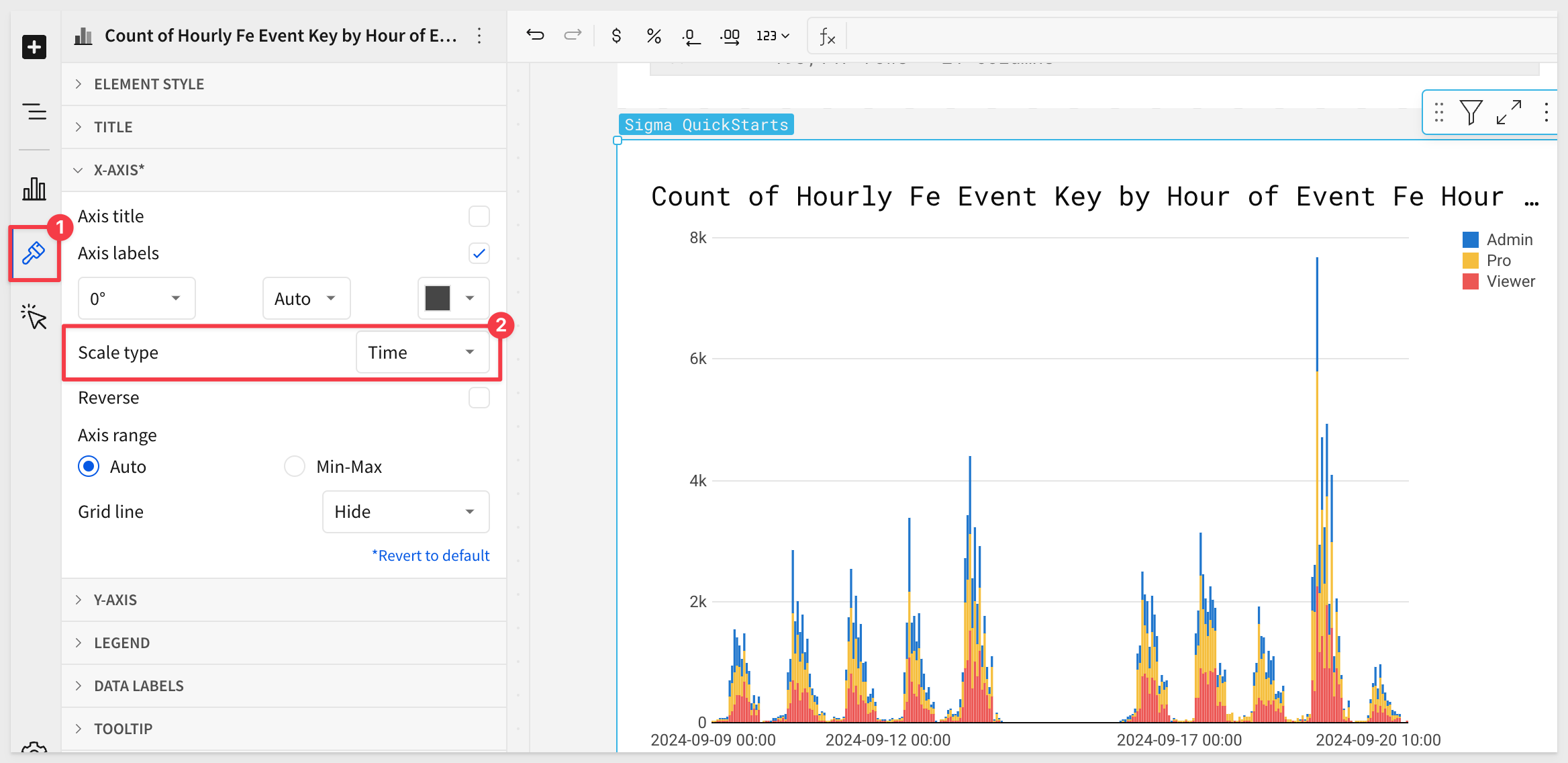
4.18 Click the paint brush icon in the lefthand panel. Select X-Axis and change scale type to Time:
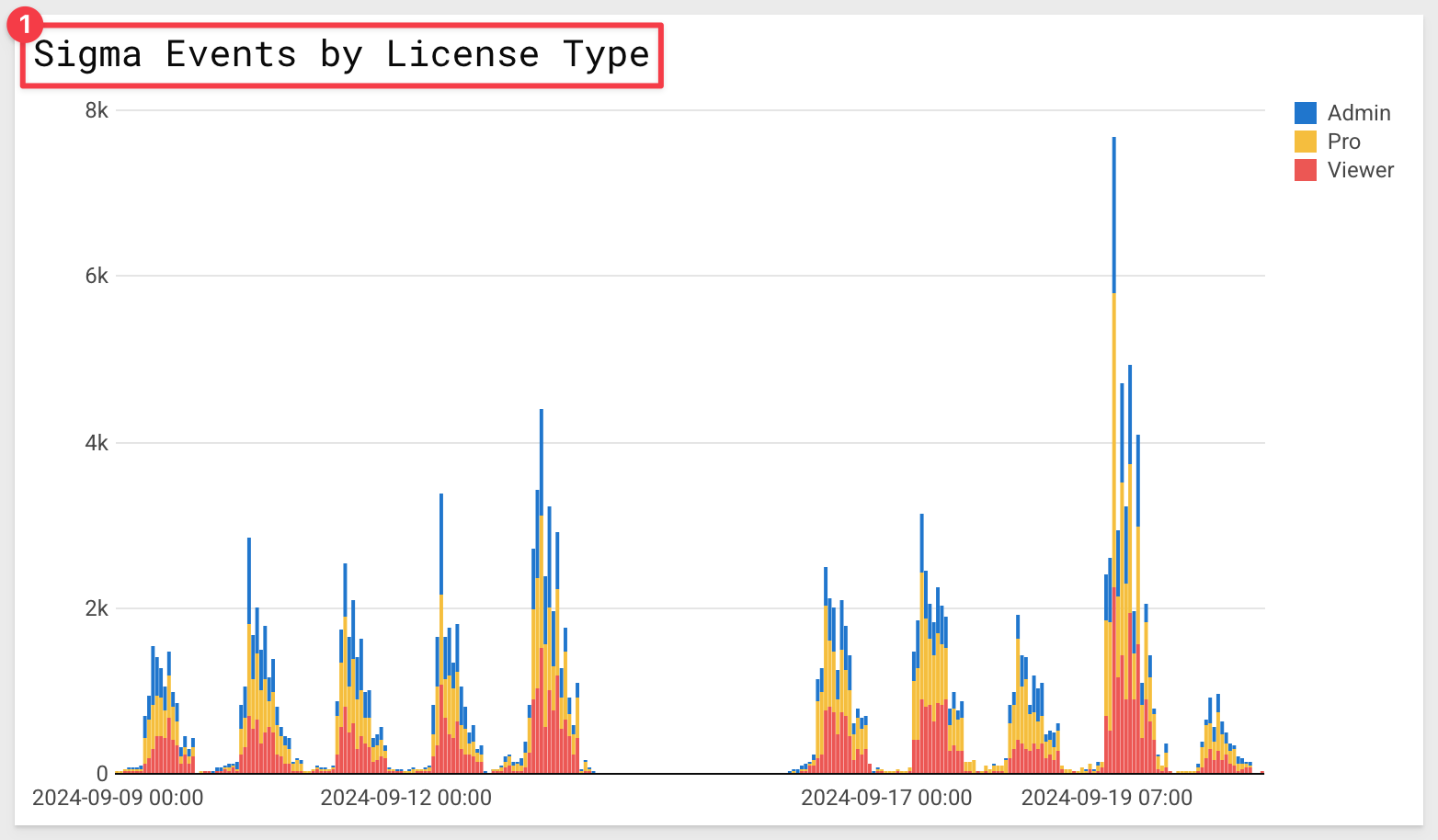
4.19 Finally, Double click the chart title and rename it Sigma Events by License Type:
4.20 Drag the new chart directly below Snowflake Queries by Day & Warehouse:
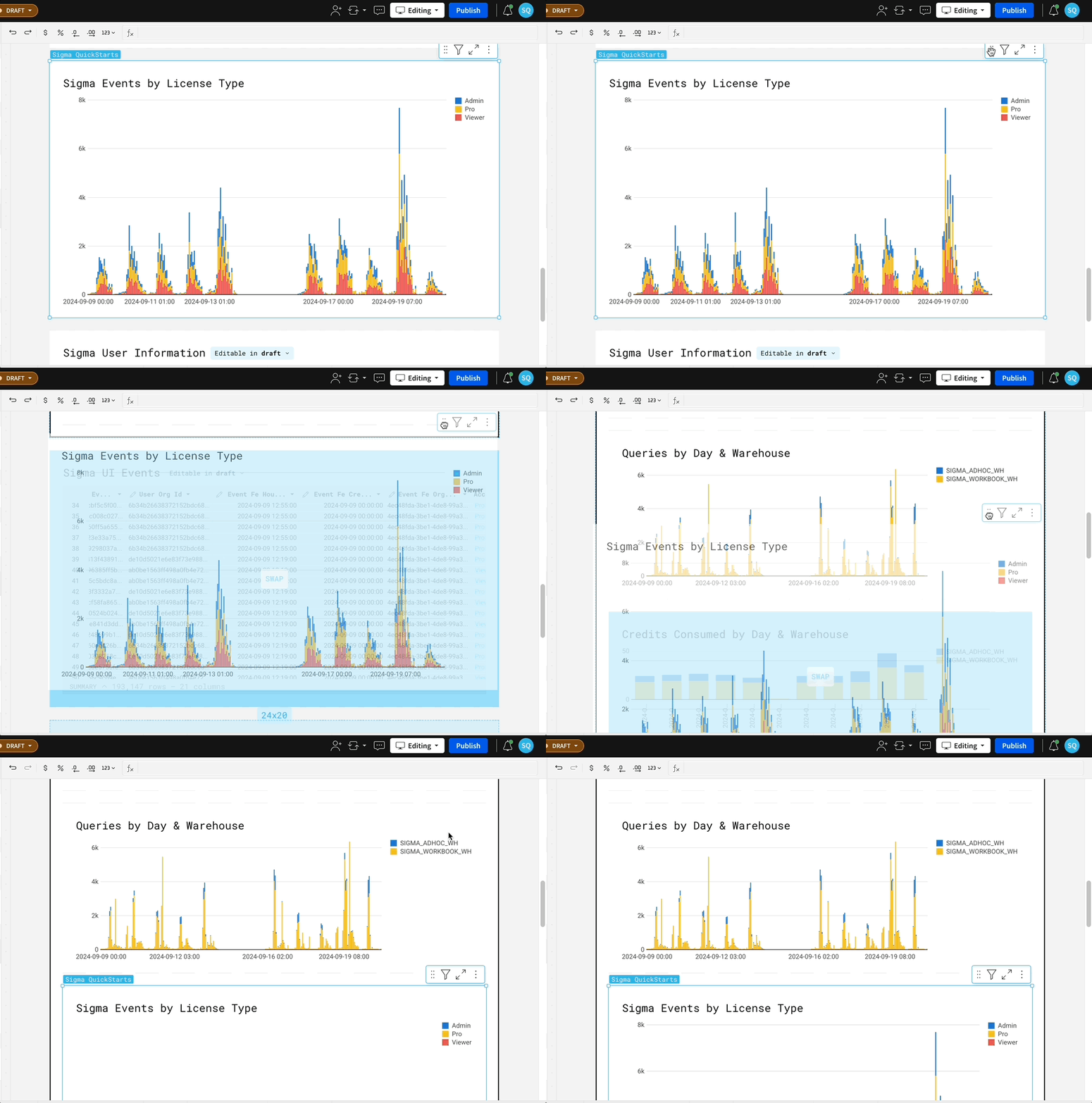
You will notice that the number of Snowflake queries from the Sigma Warehouse sometimes exceeds the number of Sigma UI Events.
This is due to the fact that Sigma fires queries against the metadata in the cloud services layer to index catalogs, schemas, tables, and views.
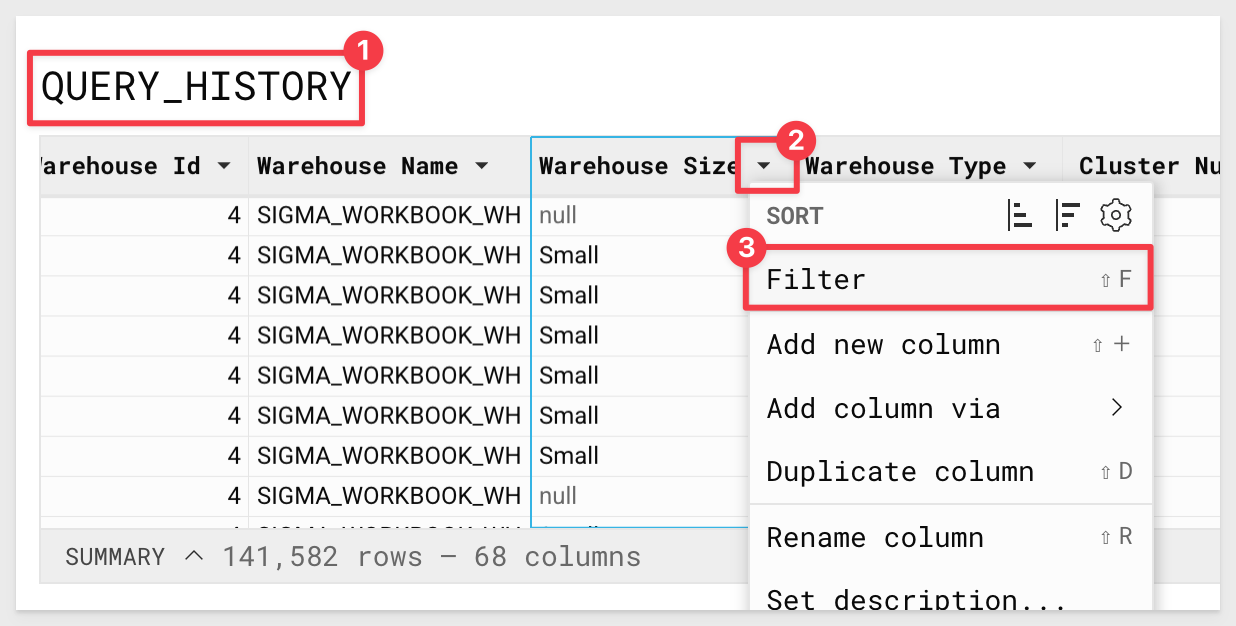
4.21 To narrow the data down to only show queries where an active warehouse was leveraged, navigate to the Query History table.
Scroll through the query history table until you see the column Warehouse Size.
Select the down arrow next to this column and select Filter:
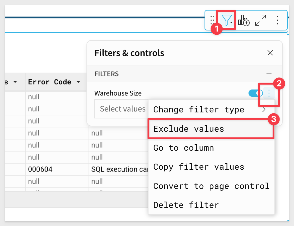
4.22 Select the three dots next to the filter, and select Exclude Values:
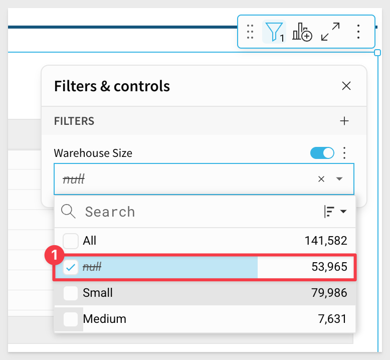
This filter will now exclude any values selected:
4.23 Using the filter, select Null to remove any queries from the dataset that did not require a running warehouse.
We can now see that the UI Events exceed queries where the warehouse was active.
This is because Sigma has built in optimizations that allow it to leverage the results cache in Snowflake, as well as execute some operations in browser to avoid unnecessary compute on the warehouse:
4.24 Now that we have a sense of usage trends, we want to start exploring how user count is impacting credit consumption.
On the Warehouse Metering History table, find the column Start Time.
Click the down arrow, and select Truncate Date > Day:
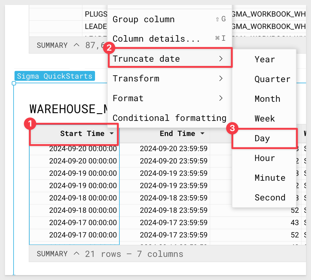
4.25 Select the drop down next to the new Day of Start Time column and click Group Column:
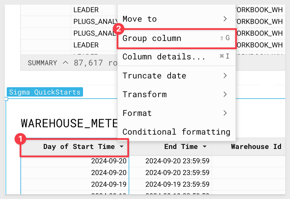
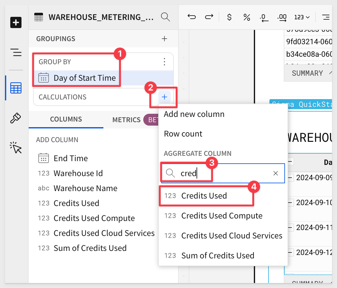
4.26 Now that the data is grouped based on the day, click the + in the Day of Start Time group, search for Credits Used and select that:
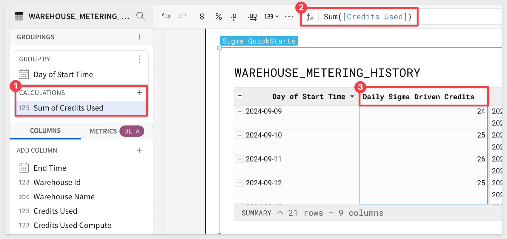
4.27 Sigma automatically summed the Credits Used for us:
Rename this column to Daily Sigma Driven Credits:
4.28 Next, scroll down to the Sigma UI Events table.
We are going to create a "stable table" off of this input table for analysis, as some functionality is not currently available on input tables directly.
Hover over the top right, select Create Child Element, then select table.
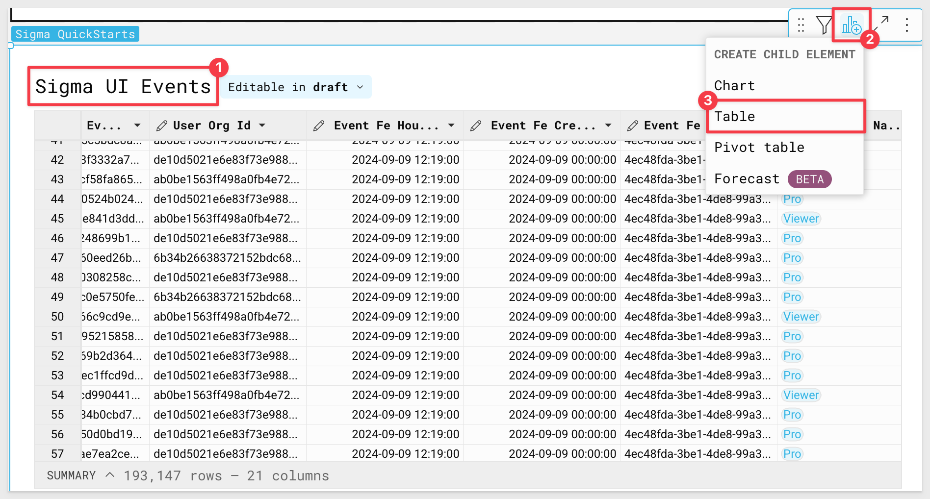
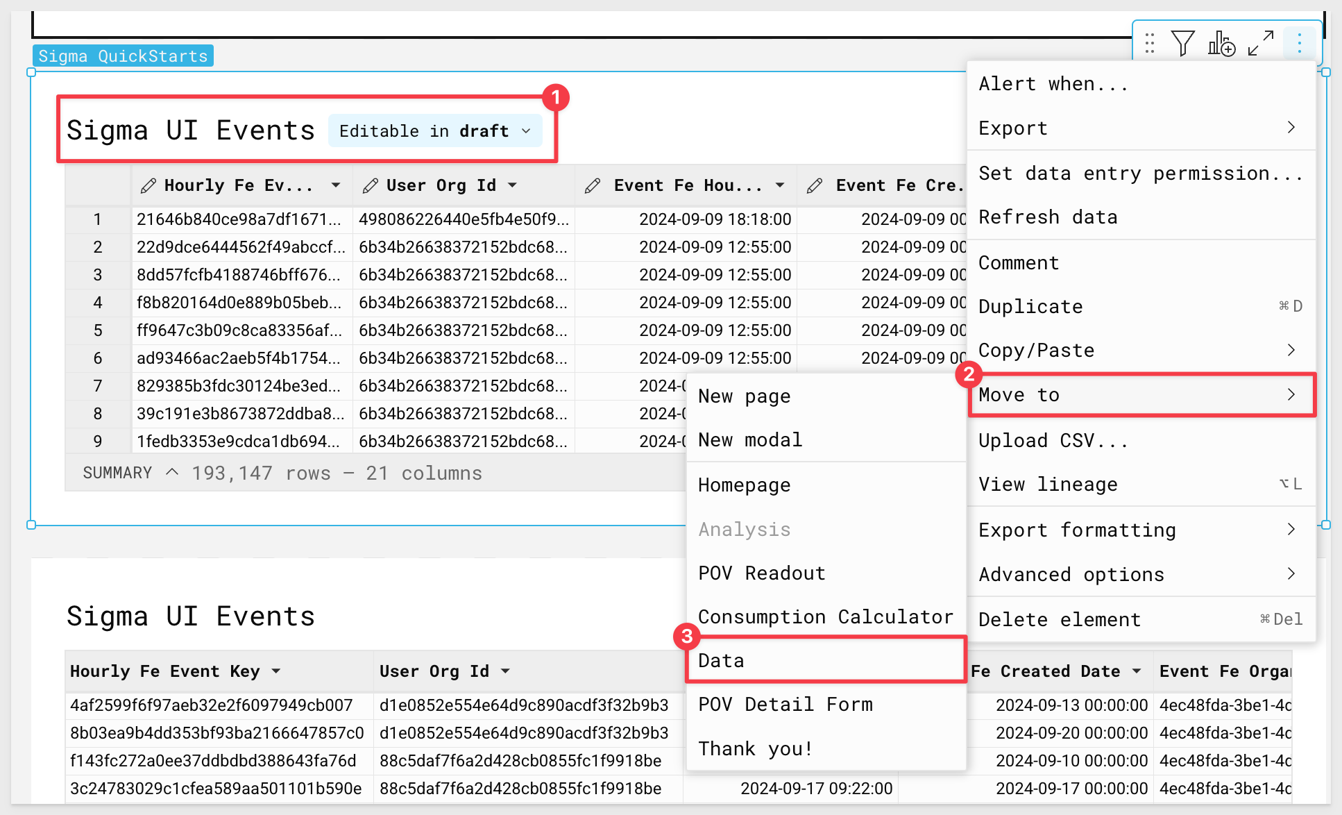
4.29 To keep our workspace clear, move the input table version (the table with pencils in each column header) to the data page by selecting the three dots in the top right hand and selecting Move to > Data:
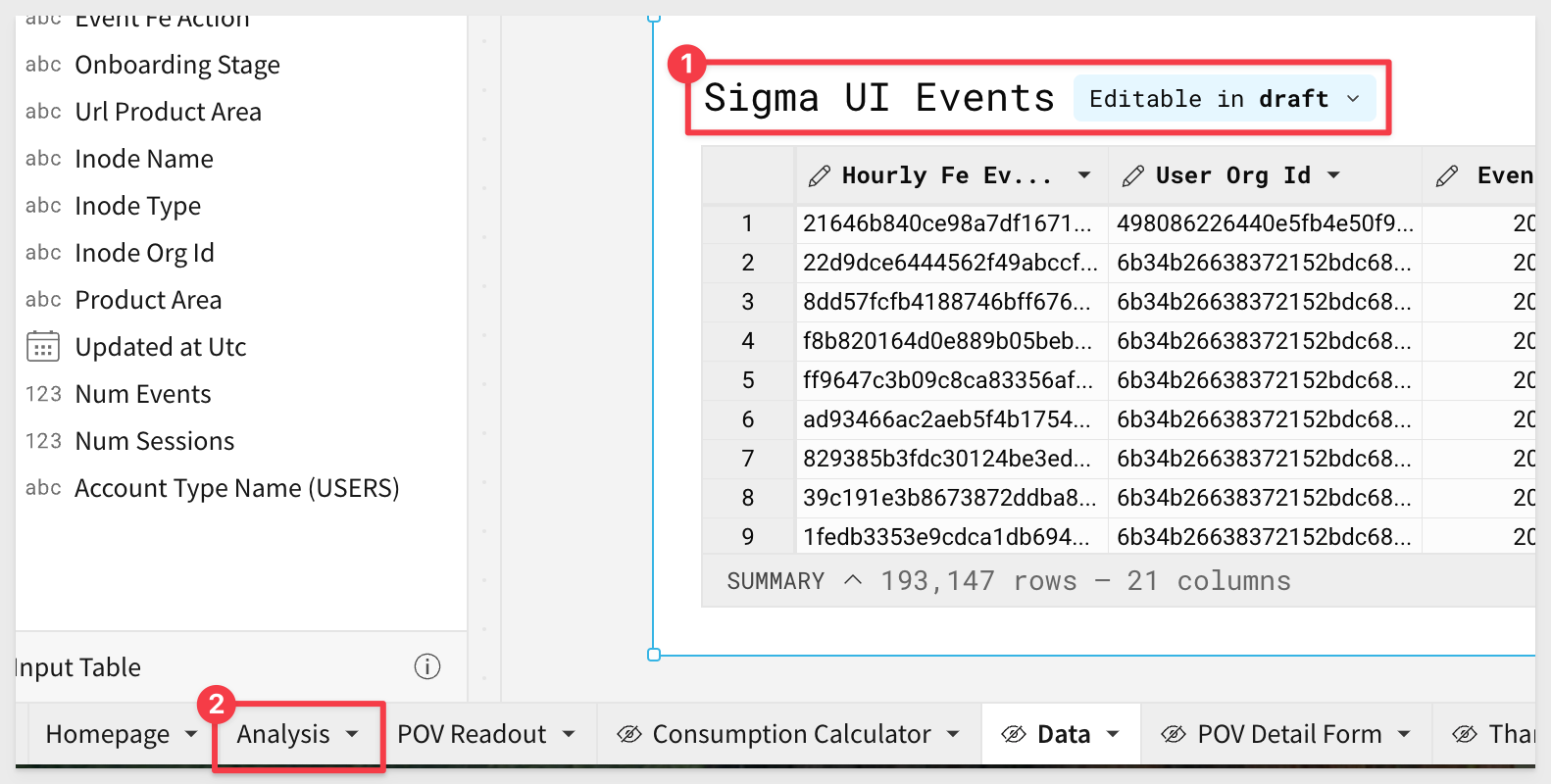
4.30 Navigate back to the analysis page using the tabs on the bottom:
4.31 Return to the Sigma UI Events stable table.
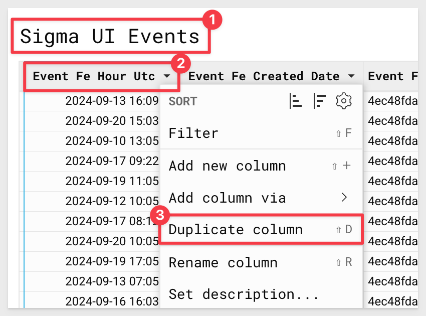
We are going to leverage this table to understand the portion of events driven by each user of each license type at the workbook level, and tie that back to credit burn.
Find the column labeled Event Fe Hour UTC, select the drop down and click Duplicate Column:
4.32 Rename this new column Day:
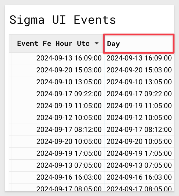
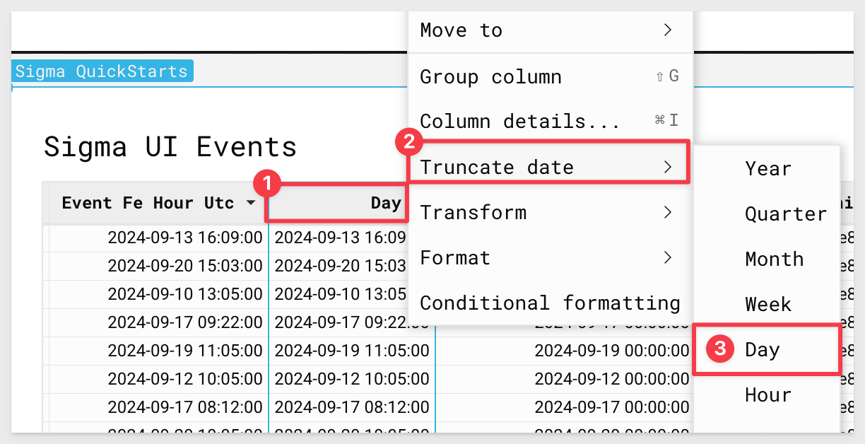
4.33 Select the down arrow next to the new Day column and select Truncate Date > Day:
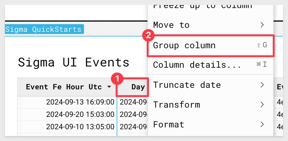
4.34 Finally, select the drop down next to Day once more and select Group Column:
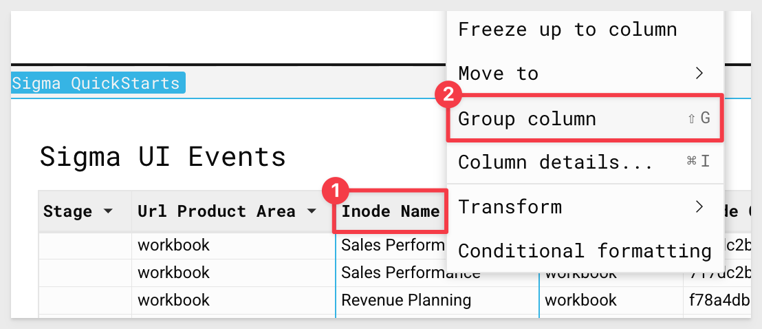
4.35 Next, find the column labeled Inode Name and group on this column:
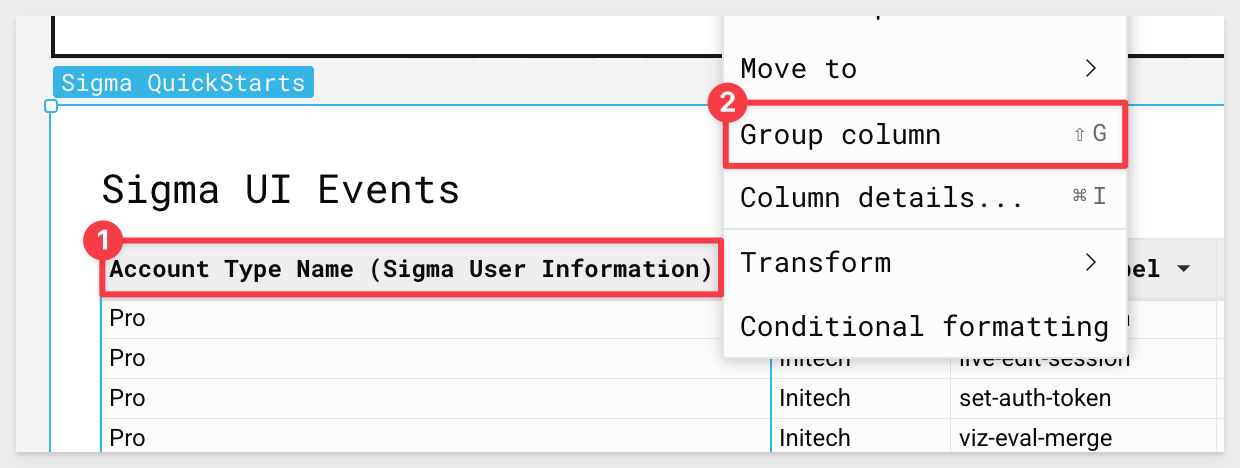
4.36 Finally, create a third level of grouping using the column Account Type Name (Sigma User Information) that was added to the table previously, via look up.
Selecting the drop down and click Group Column:
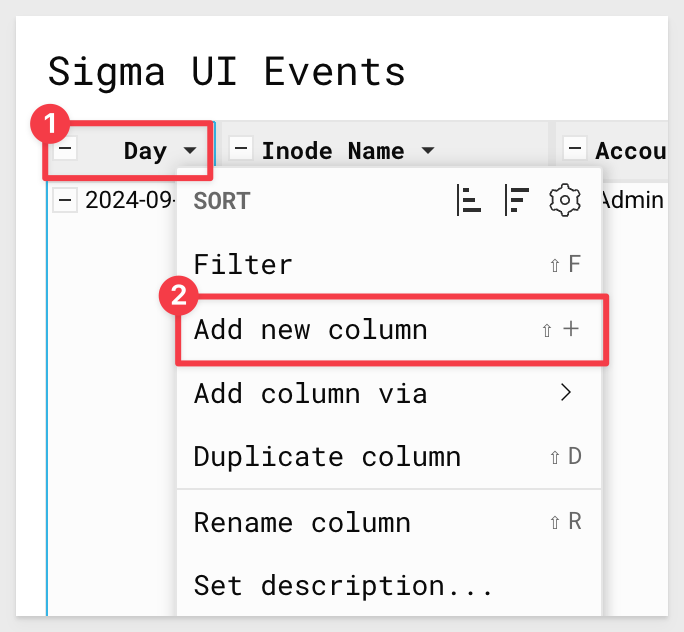
4.37 Now that we have the data aggregated at several levels, we are going to start calculating usage at these aggregates.
Select the drop down next to the first grouping on Day, and select Add New Column:
4.38 In the formula bar, type:
CountDistinct([Hourly Fe Event Key])
```

Rename this column `Daily Events`:

<img src="assets/nasa-3-38.png" width="600"/>

4.39 Click the drop down next to the new `Daily Events` column and select `Duplicate Column`:

<img src="assets/nasa-3-39.png" width="400"/>

4.40 Once again click the drop down and duplicate the column two more times, so that you have three columns, `Daily Events`, `Daily Events (1)`, and `Daily Events (2)`:

<img src="assets/nasa-3-40.png" width="800"/>

4.41 Using the UI menu on the lefthand side, drag `Daily Events (1)` under the `Innode Name` grouping.

Double click `Daily Events(1)` and rename the column `Workbook Events`:

<img src="assets/nasa-3-41.png" width="800"/>

4.42 Next, drag `Daily Events(2)` from the `Day` grouping to the grouping under `Account Type Name` in the lefthand panel.

Rename `Daily Events (2)` to `WB Events by License Type`:

<img src="assets/nasa-3-43.png" width="400"/>

4.43 Click the drop down next to the new `Daily Events` column and select `Add new column Via Lookup`:

<img src="assets/nasa-3-45.png" width="700"/>

4.44 We want to look up to the `WH Metering History` table.

For columns to add, select `Daily Sigma Driven Credits`.

Finally, map the columns on `Day = Day of Start Time` and click `Done`:

<img src="assets/nasa-3-46.png" width="400"/>

4.45 Rename this new column `Daily Credits`:

<img src="assets/nasa-3-47.png" width="600"/>

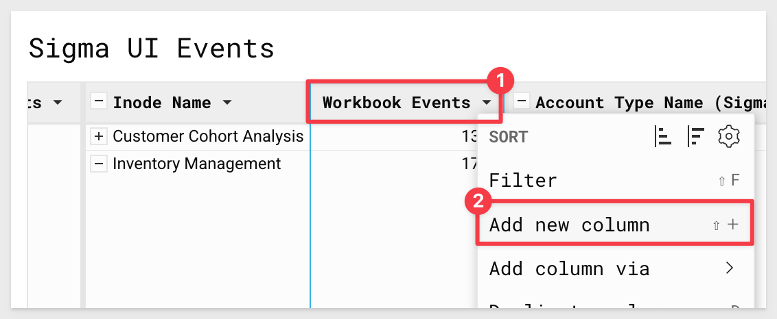
4.46 At the next grouping on `Inode Name`, click the down arrow by `Workbook Events` and click `Add new Column`.

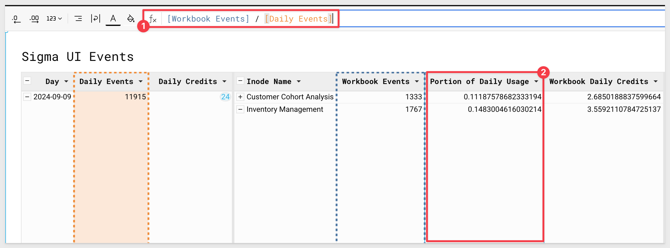
In the formula bar, enter
```copy-code
[Workbook Events]/[Daily Events]
Rename this new column Portion of Daily Usage:
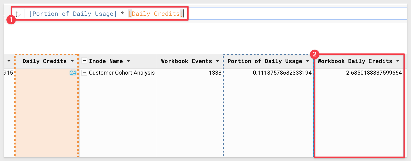
4.47 Finally, add one more column off of Portion of Daily Usage.
In the formula bar, type:
[Portion of Daily Usage] * [Daily Credits]
Rename this column Workbook Daily Credits:
4.48 At the Account Type Name grouping, add a new column off of WB Events by License Type:
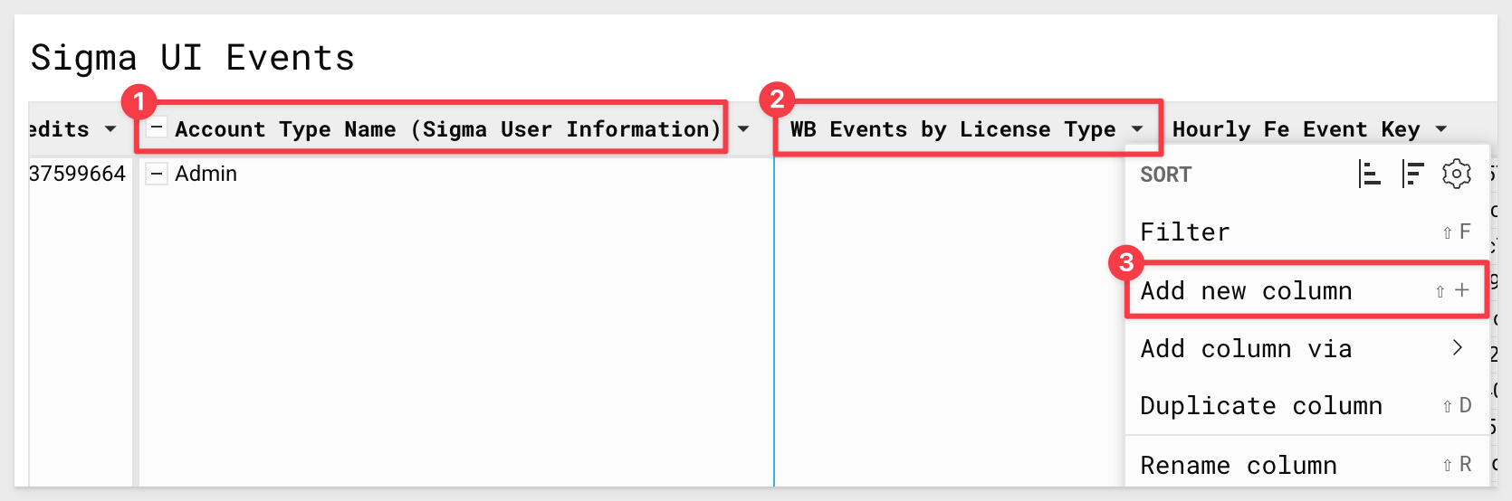
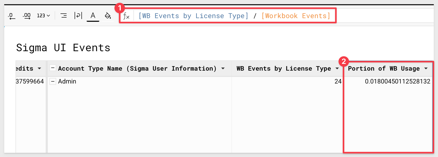
In the formula bar enter:
[WB Events by License Type]/[Workbook Events]
Rename this new column Portion of WB Usage:
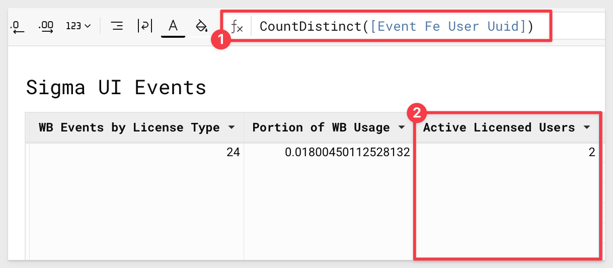
4.49 Next, add a new column off of Portion of WB Usage and set the formula to:
CountDistinct([Event Fe User Uuid]).
Rename this column Active Licensed Users:
4.50 Finally, add one last column to the right of Active Licensed Users.
Set the formula bar to:
([WorkBook Daily Credits]*[Portion of WB Usage]) / [Active Licensed Users]
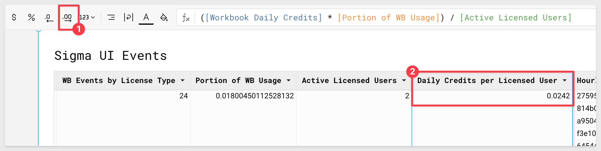
Rename this new column Daily Credits per Licensed User:
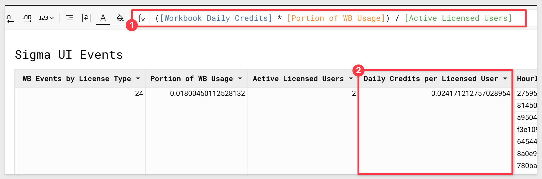
4.51 Using the buttons next to the formula bar, adjust the decimal places so that the value is four characters past the zero:
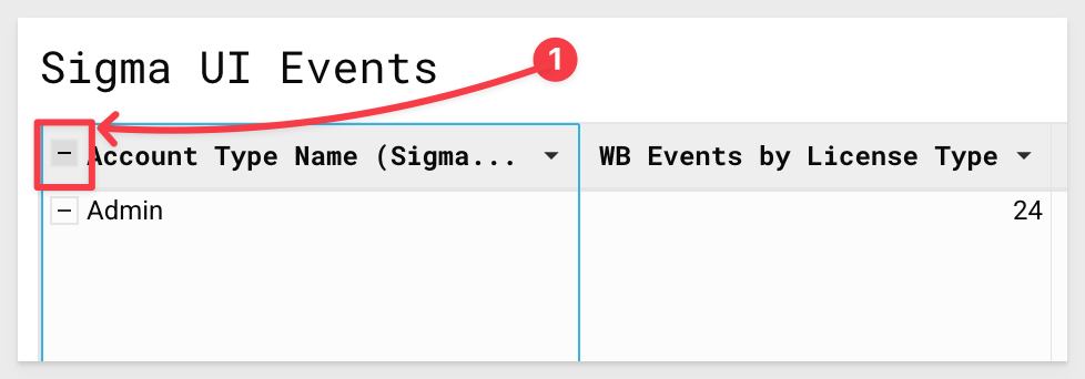
4.52 Click the minus symbol next to the Account Type Name grouping to collapse the table at this level:
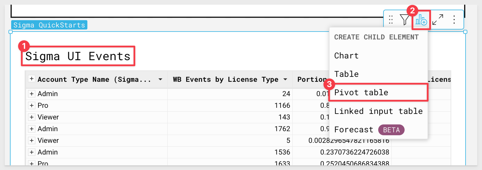
4.53 On the Sigma UI Events table, in the upper righthand side, click and select Create Child Element, then Pivot Table:
4.54 For pivot rows, select Inode Name.
For columns, select Account Type Name, and for values, use Daily Credits Per Licensed User:
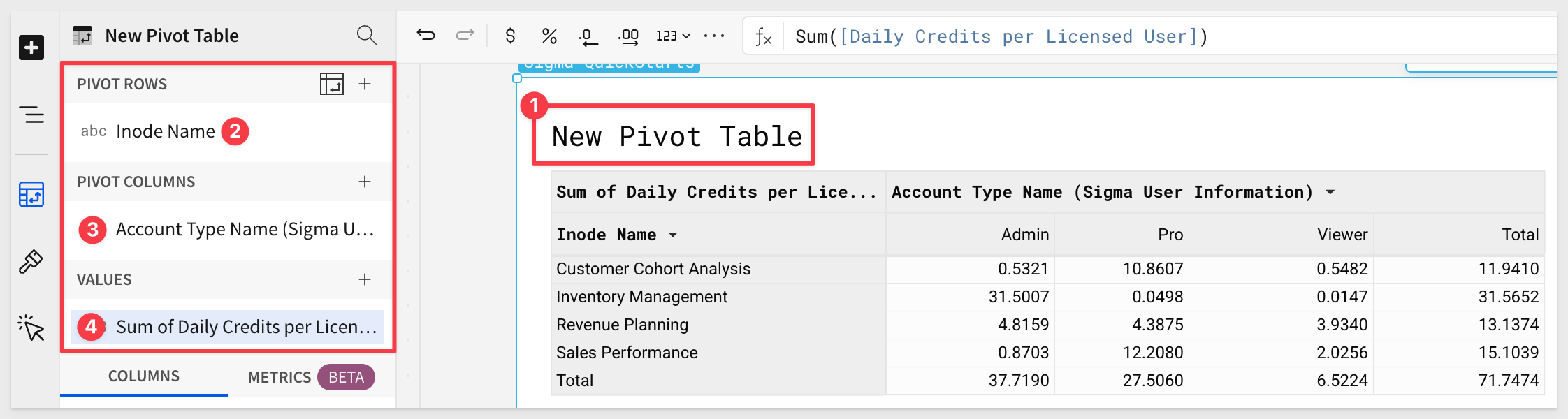
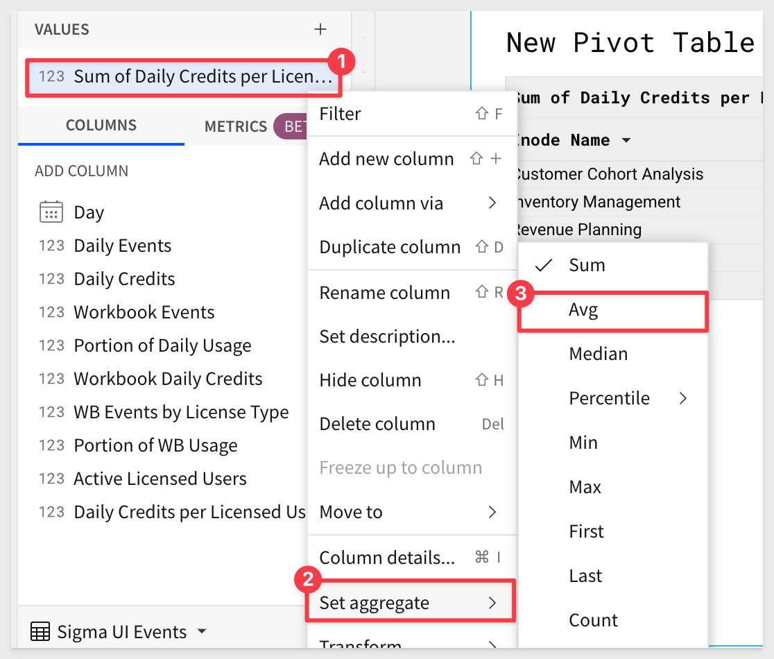
4.55 You will notice Sigma automatically Sums the Daily Credits column.
Change the aggregate for this value to Average, by clicking the drop down, Set Aggregate, then AVG:
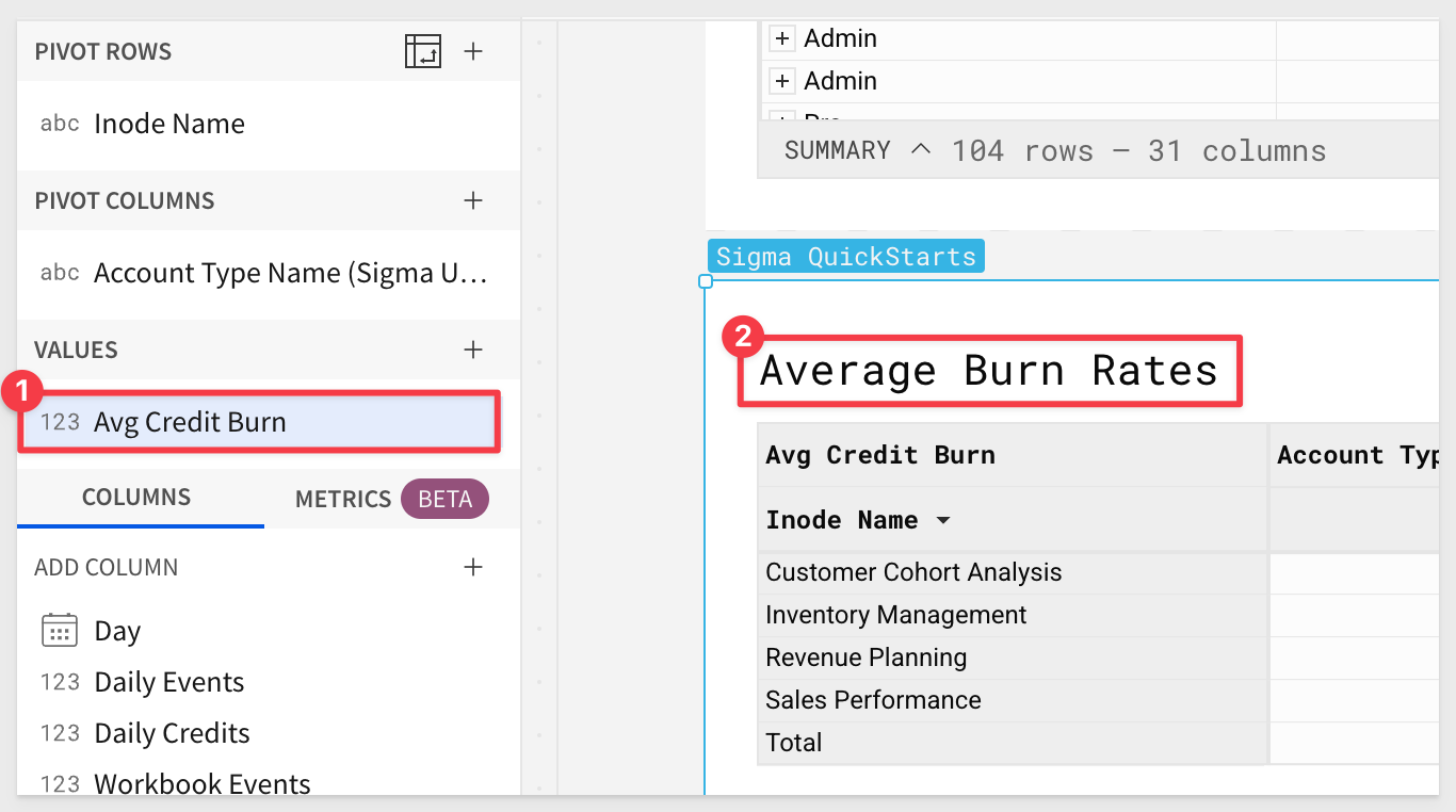
4.56 Rename the average value to Avg Credit Burn.
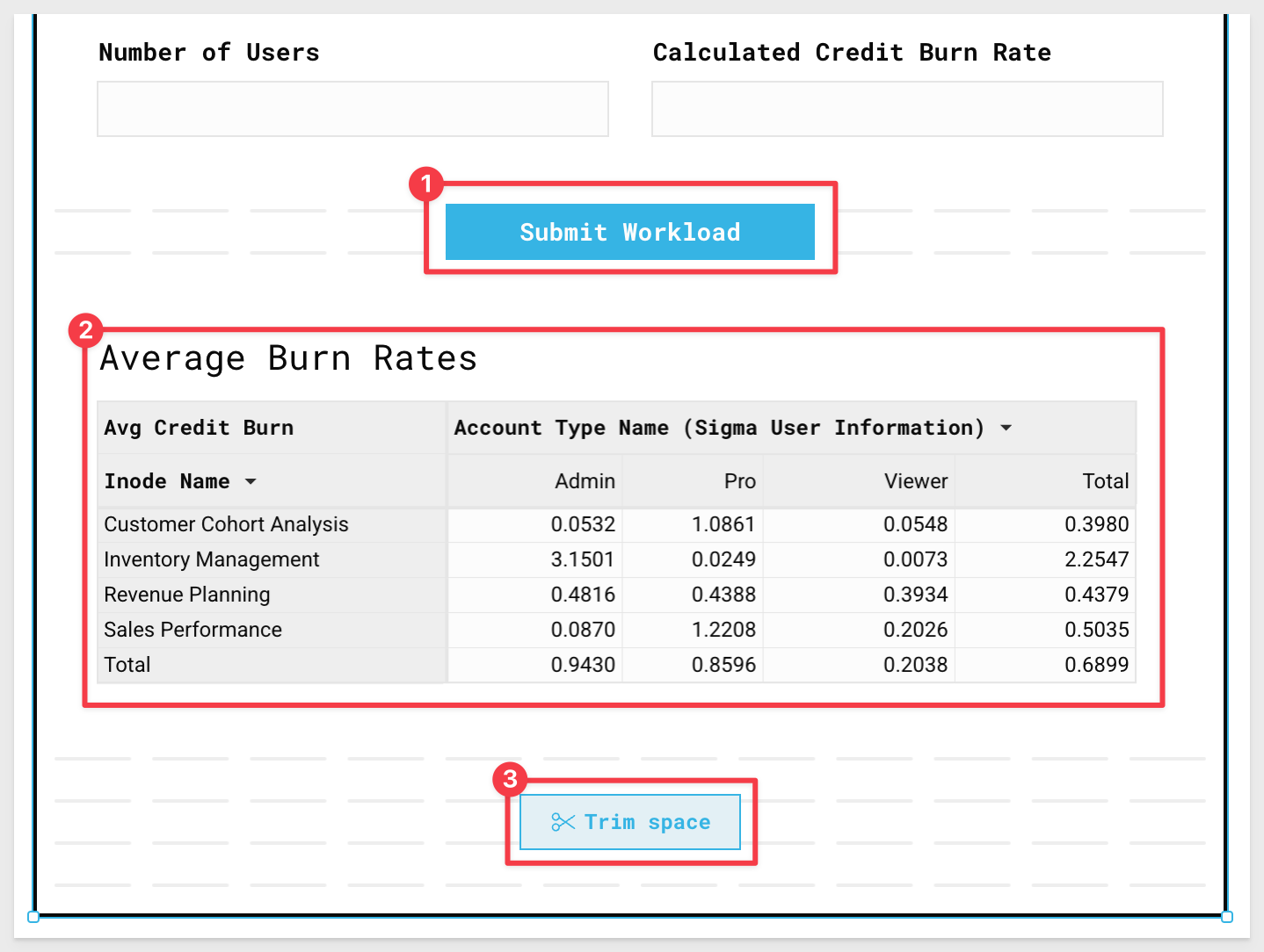
Also rename the pivot table Average Burn Rates by double clicking the title.
We can now see the average daily credit burn against the different workloads by users of the different license types.
We can take this information and leverage the Consumption Calculator within the workload to extrapolate the yearly credit burn for the customers anticipated workloads and user counts:
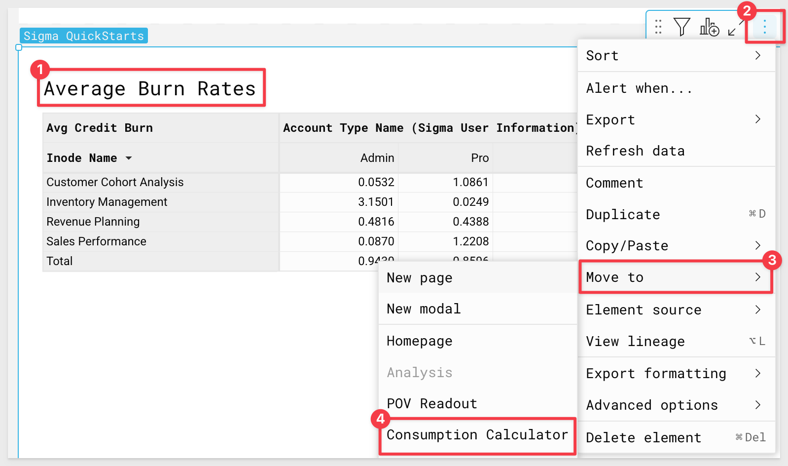
4.57 Click on your pivot table, then select the three dots.
From the menu, select Move to and then Consumption Calculator:
4.58 Drag the pivot table so that it sits directly below the Submit Workload button:
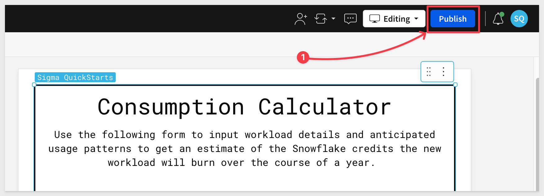
4.59 At the top of the page, click the blue Publish button to save your work:
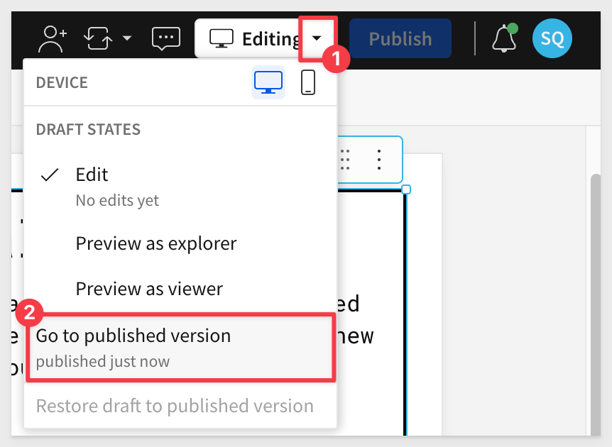
5.1 Click the drop down next to the white Editing button and click Go to Published Version:
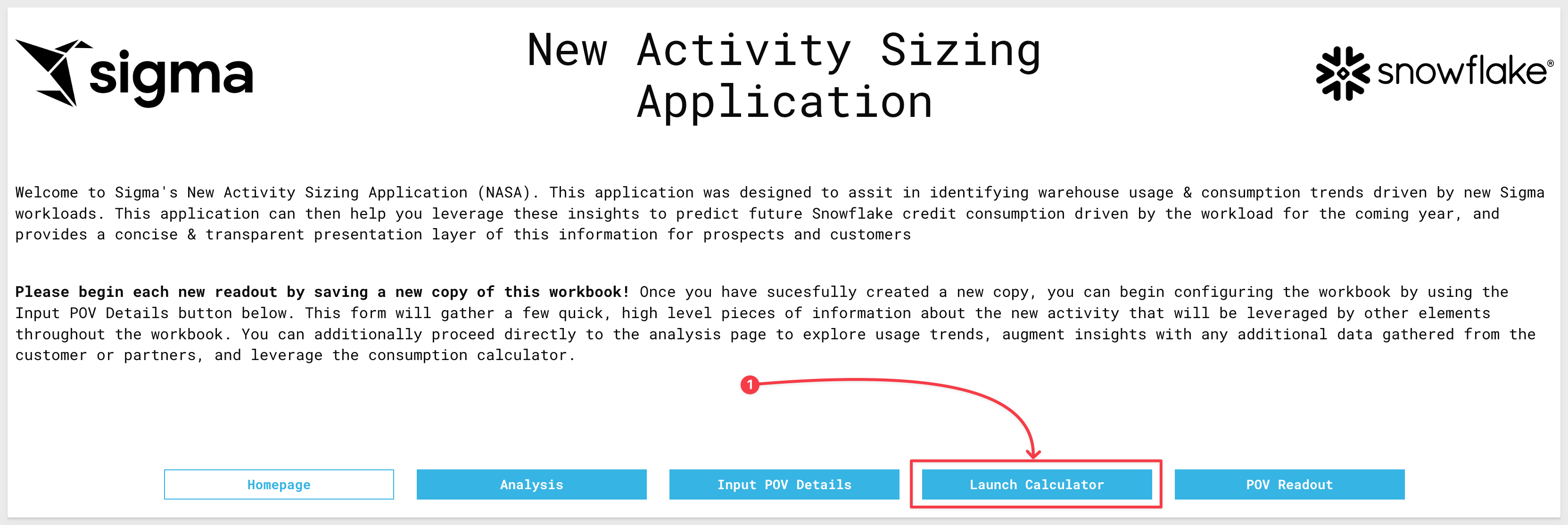
5.2 Click the blue Launch Calculator button in the workbook header:
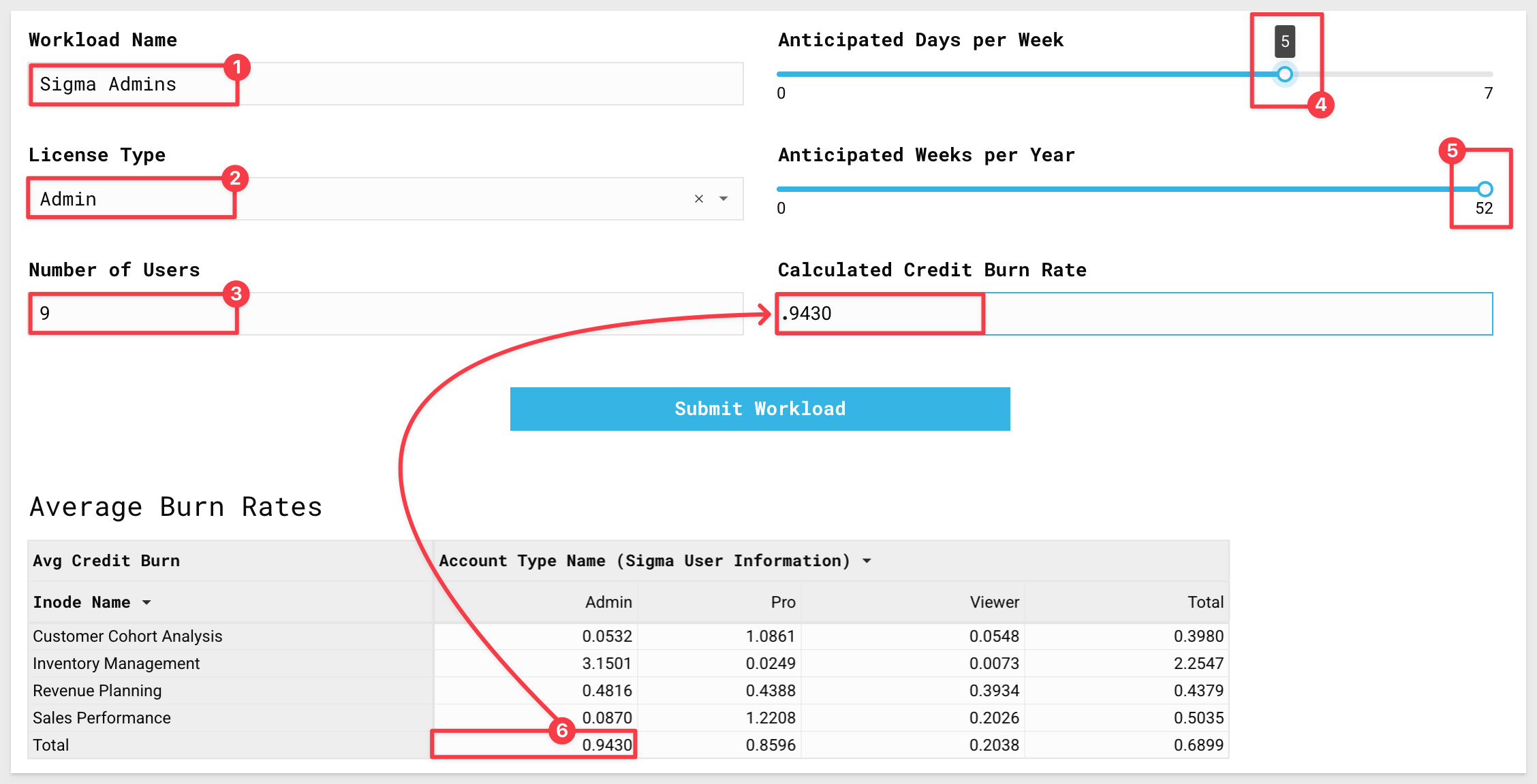
5.3 For workload name, type Sigma Admins.
For License type, select Admin from the drop down.
For number of users, enter 9.
For days per week, slide the selection bar to 5.
For weeks per year, slide the selection bar to 52.
For Calculated Workload Credit Burn for License Type enter the value you see under Admin in the Total at the bottom (see screenshot below...).
We are leveraging the daily average across all workloads for the admin users, as their work is not typically tied to a single workbook.
Click Submit Workload:
5.4 Prepare another workload by entering Customer Cohort Pro as the workload name.
For License type select Pro.
For number of users enter 20.
Anticipated Days per Week will be 5.
Weeks per Year being 52.
Finally, for Calculated Credit Burn Rate, enter the value you see for Customer Cohort Analysis under Pro in the pivot table:
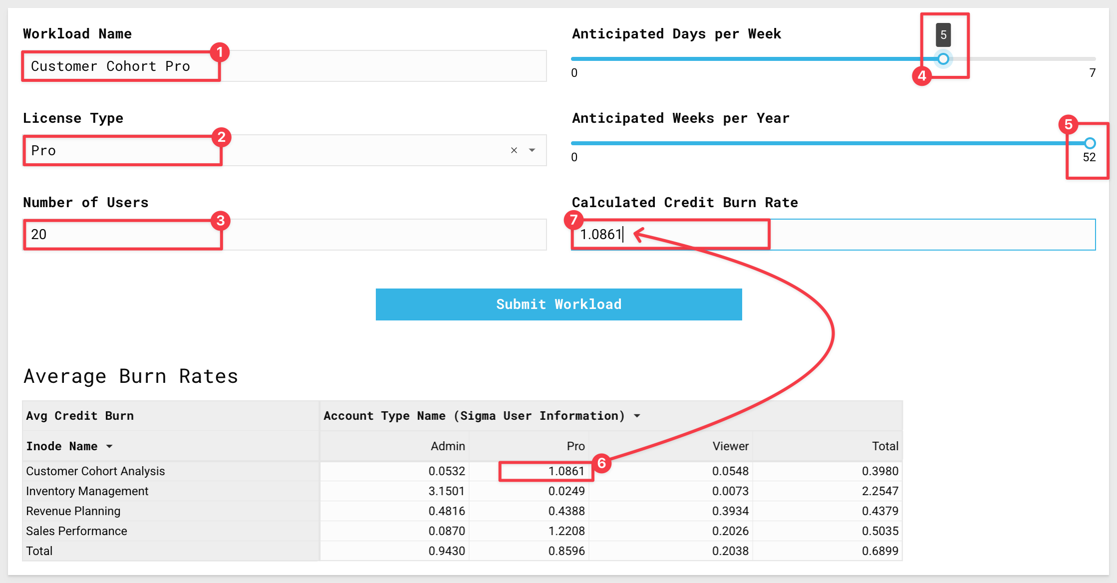
Click Submit Workload.
5.5 Finally, enter Customer Cohort Viewer as the workload name.
For license type, select Viewer.
For anticipated number of users, enter 50.
Assume 5 days a week, 52 weeks per year.
Finally, for Calculated Credit Burn value enter the value you see for Customer Cohort Analysis under Viewer:
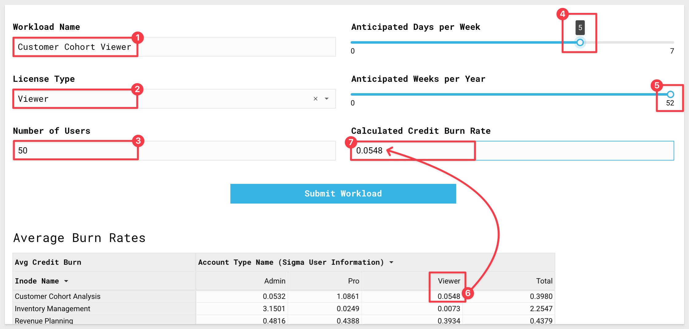
Click Submit Workload.
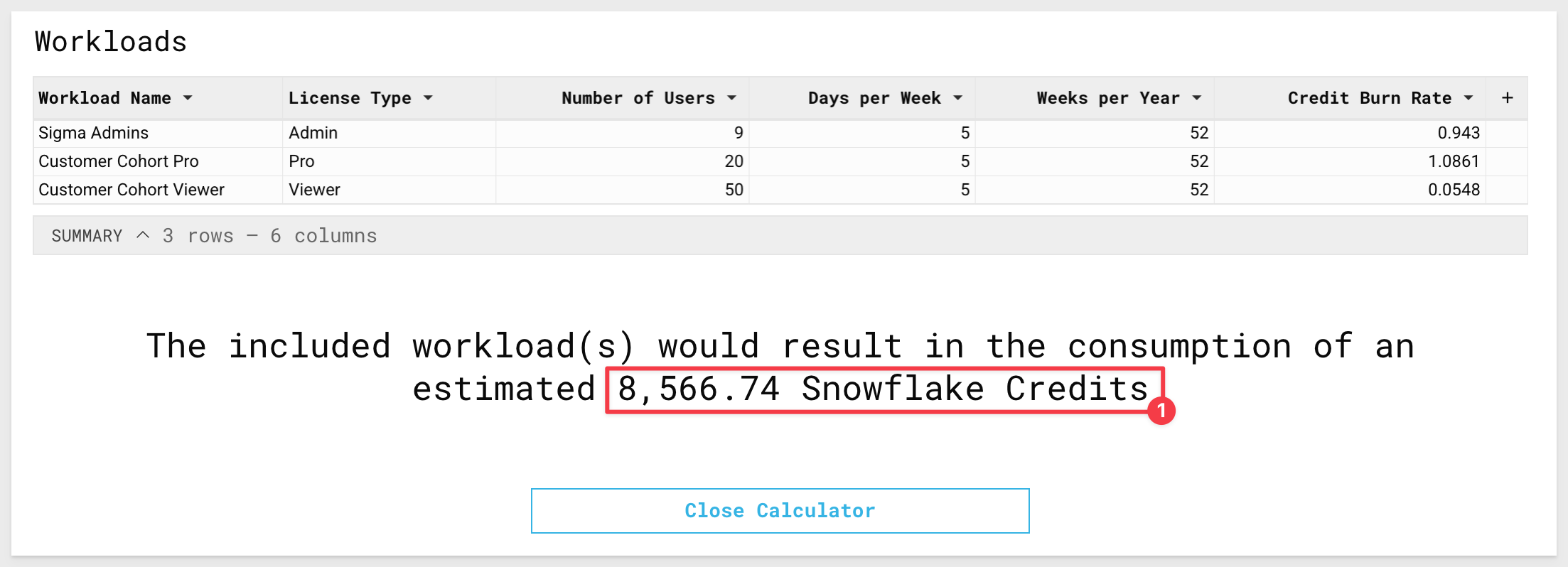
5.6 We have used the calculator to create three workloads.
Scroll to the bottom of the calculator.
You will see a table holding the submitted workloads, as well as the final credit consumption number associated with the inputs:
5.7 Click the Close Calculator button.
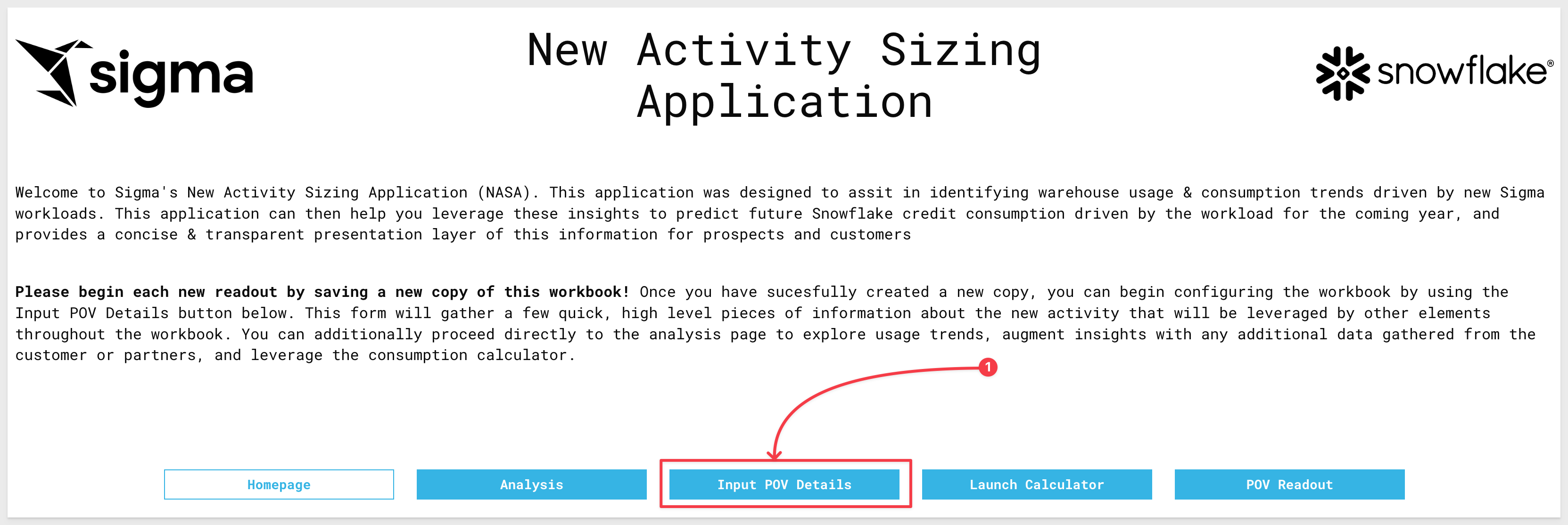
6.1 From the Homepage click the Input POV Details button to open the POV Detail Form:
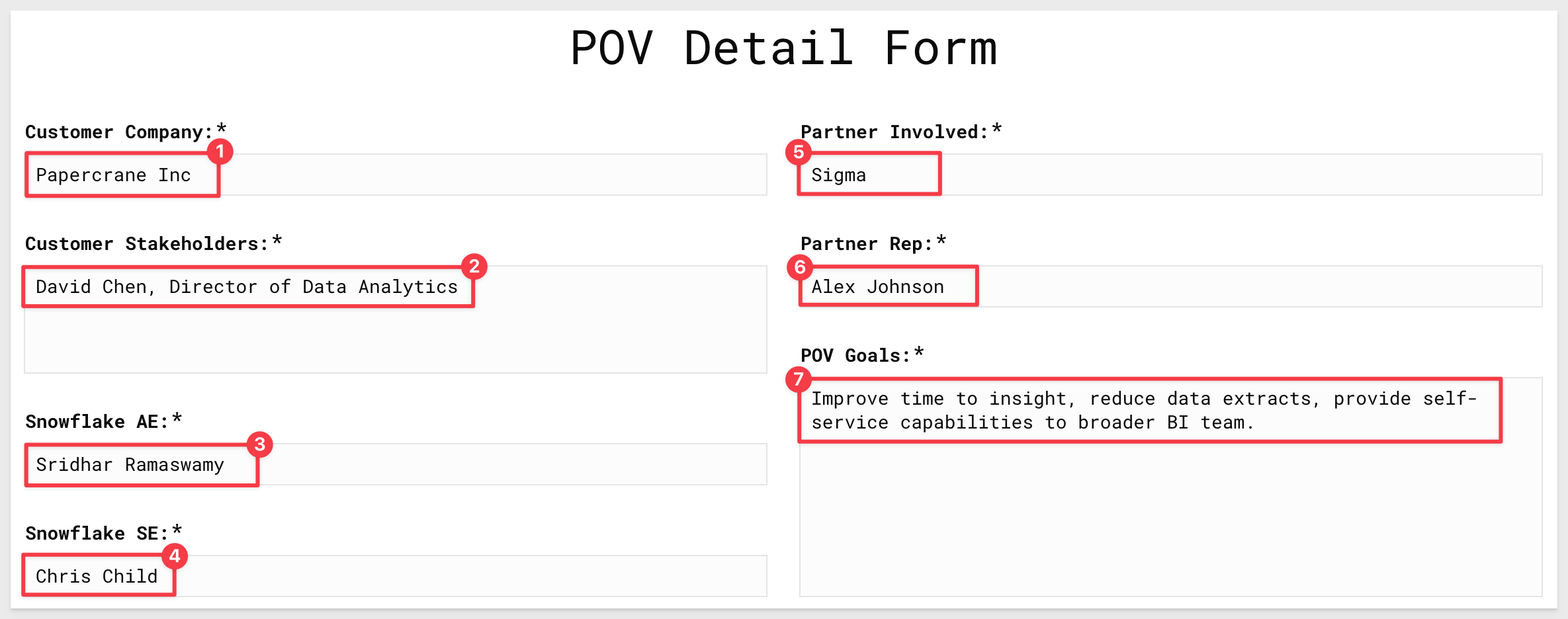
6.2 For Customer Company, type Papercrane Inc.
In Stakeholders, enter David Chen, Director of Data Analytics.
You may enter any combination of names for Snowflake AE and Snowflake SE.
For Partner Involved type Sigma.
For Partner Rep, type Alex Johnson.
Finally, for POV Goals, copy and paste the following:
Improve time to insight, reduce data extracts, provide self-service capabilities to broader BI team
6.3 Click Submit on the POV Detail Form.
Click Close on the Thank you! modal:
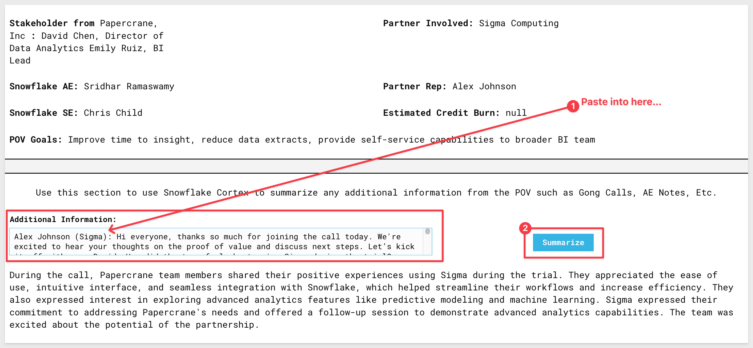
6.4 Finally, copy the text from the POV_Readout_Gong_call.txt file that was included in the zip file we downloaded earlier.
Paste the text into the Additional Information box on the screen and click Summarize.
This will call Snowflake Cortex to summarize the Gong transcript and return highlights from Papercrane's Sigma POV:
In this QuickStart, we used Sigma to provide a detailed readout of POV activity and a data-backed prediction of future usage for your customer.
Additional Resource Links
Blog
Community
Help Center
QuickStarts
Be sure to check out all the latest developments at Sigma's First Friday Feature page!