A discounted cash flow (DCF) is an analysis that values some type of asset over a period of time.
More simply put, it allows someone to understand how much future money is worth in today's terms.
Historically, this type of analysis has been done in traditional spreadsheet tools like Excel. While a reliable tool, financial analysts and accountants often encounter challenges when performing a DCF in Excel:
- Scalability Issues: Large datasets must be rolled up/aggregated to fit within Excel's ~1 million row limit, leading to a loss of crucial data granularity.
- Manual Updates: The process must be repeated periodically (e.g., monthly or quarterly) as new data needs to be incorporated into the original model, making it time-consuming.
- Lack of Governance: Excel lacks built-in governance features, making it difficult to prevent mistakes and ensure accuracy both proactively and retroactively.
That is where Sigma comes in.
With a familiar spreadsheet interface, Excel power users can seamlessly transition to Sigma and recreate their work in an intuitive format.
Our cloud-based architecture offers:
- Performance and Scalability: Handle datasets well beyond Excel's limits, leveraging the full compute power of your cloud data warehouse, maintaining crucial data granularity for more detailed insights.
- Automated Real-time Updates: Your DCF analysis automatically updates as new data flows into your cloud data warehouse, ensuring timely and accurate financial modeling.
- Enhanced Governance and Security: Sigma inherits all the governance features from your cloud data warehouse, including audit trails and version history, ensuring data accuracy and reducing risks associated with manual errors.
This QuickStart will provides an example of DCF, based on Sigma provided sample data, so users can build on their own.
Target Audience
Sigma users who are in a finance role or have interest in a discounted cash flow analysis.
Prerequisites
- A computer with a current browser. It does not matter which browser you want to use.
- Access to your Sigma environment.
- Some familiarity with Sigma is assumed. Not all steps will be shown as the basics are assumed to be understood.

We will be using sample data provided by Sigma, which is included with all trial and production accounts.
Workbook Setup
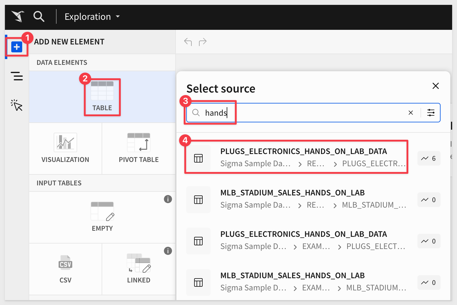
Log into Sigma and Create a new workbook.
Click the + and select TABLE; search for hands and select the PLUGS_ELECTRONICS_HANDS_ON_LAB_DATA table:
Initial Setup
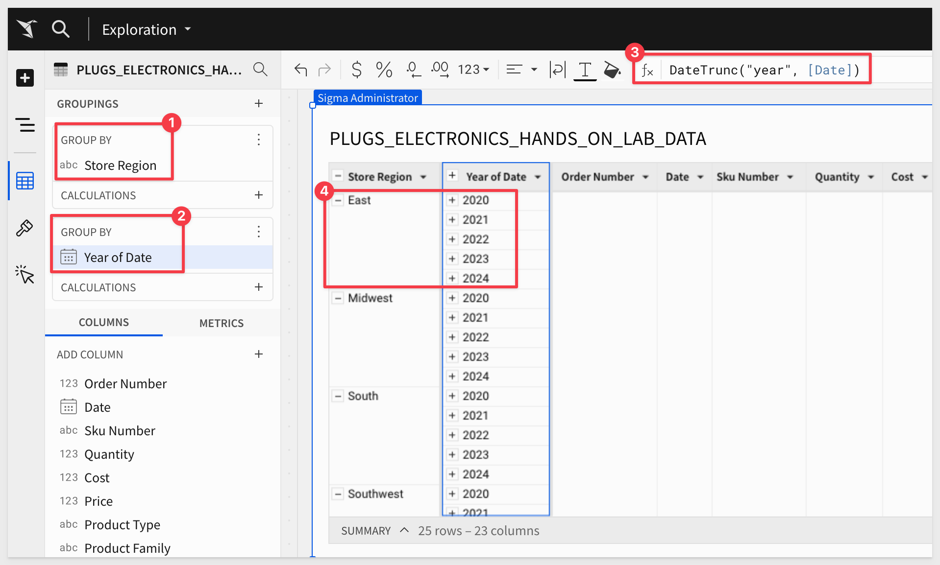
For this table, we have data from 2020 through 2024.
We want to create part of a DCF for each year, for each of the store regions.
First, we will group by Store Region and then create a second grouping on Date:
Set the formula for Date to:
DateTrunc("year", [Date])
This gives us a row for each Store Region and Year:
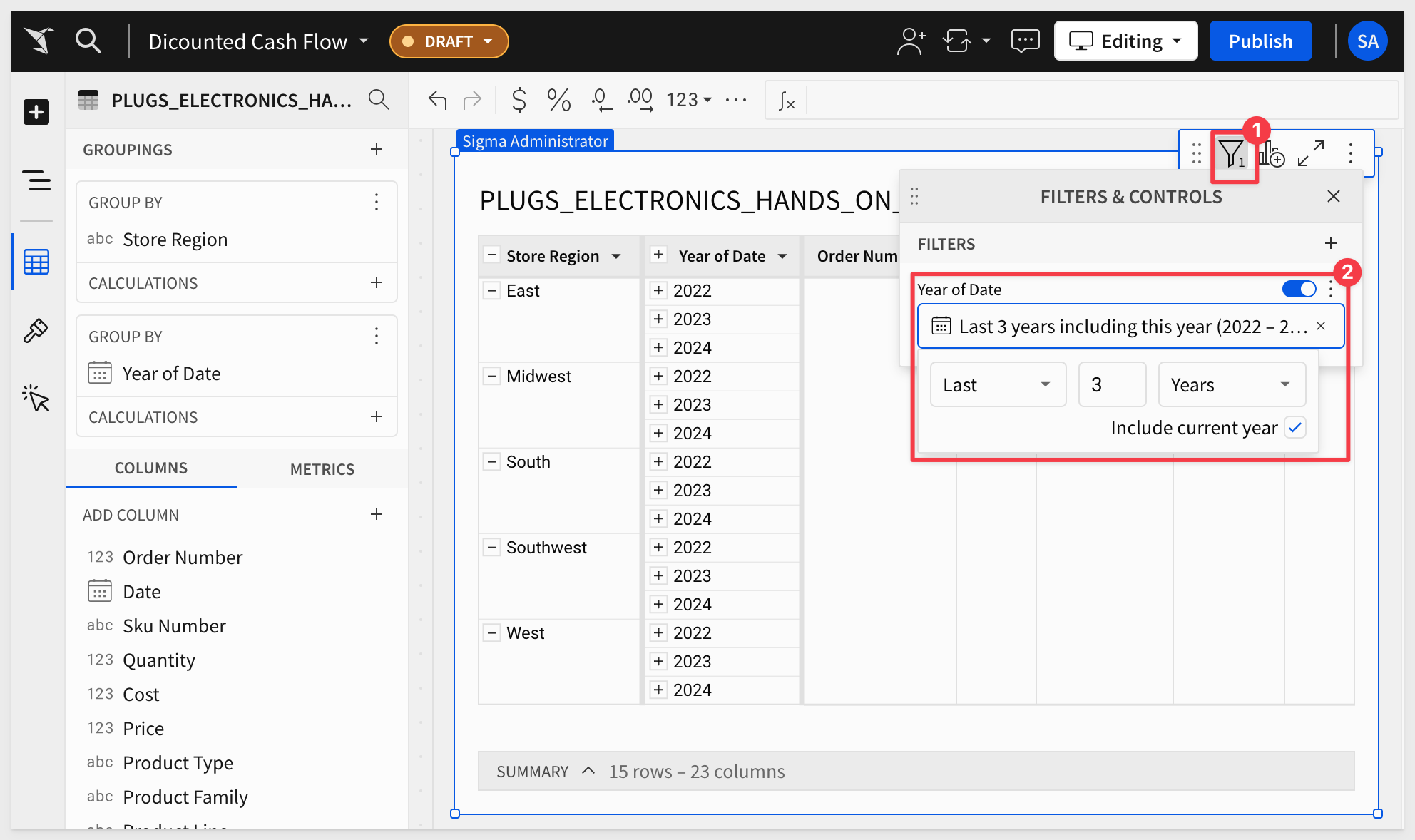
Filter on Year of Date for the last three years only:
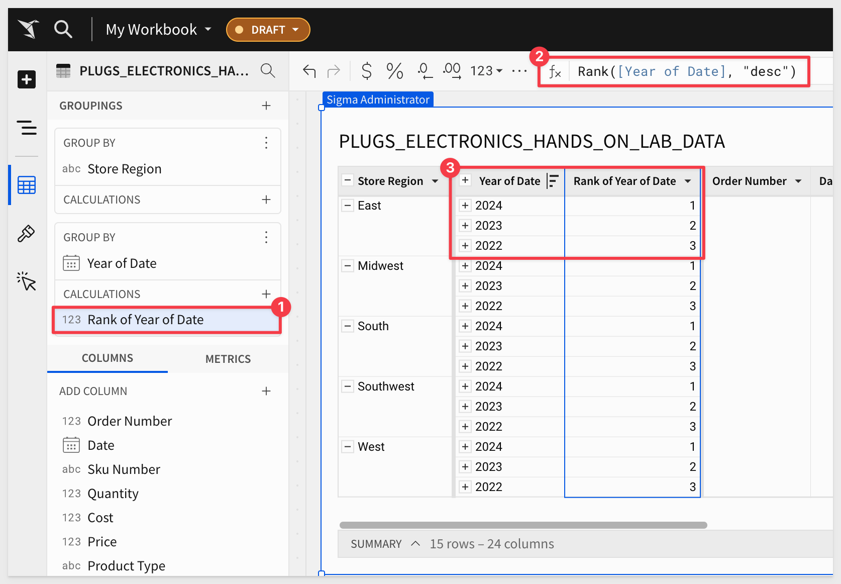
Add one more column as a CALCULATION in the Year of Date, setting its formula to:
Rank([Year of Date], "desc")
This ensures that the most recent year is always numbered as 1:
To start, we'll focus on three key components of the calculation:
- Carry Value (CV): represents the initial carrying value, which is essential for understanding the starting point of each period.
- Ending Carry Value (ECV): represents the value at the end of the period, before any reductions.
- Reduction: a change applied after establishing the beginning and ending carry values for the period.
The final step will be to calculate the actual Discounted Cash Flow (DCF) value.
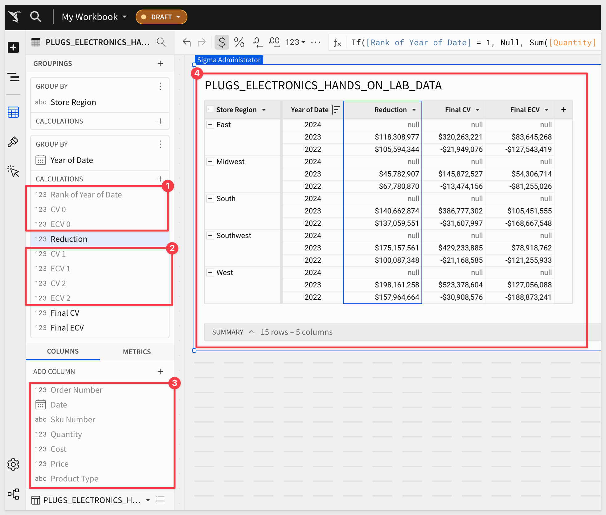
Create Columns
Add three new CALCULATION columns in the Year of Date group called CV 0, ECV 0 and Reduction.
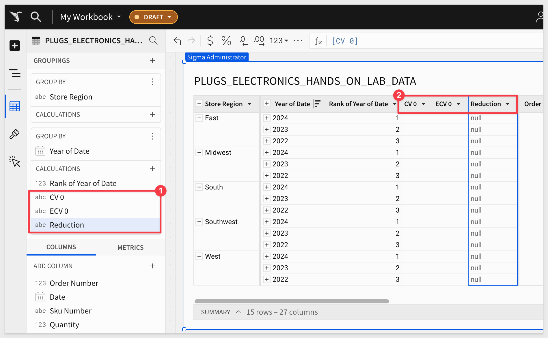
Calculate Values for the First Year
Since we're starting with the first year, there won't be any CV 0 initially. Therefore, there will only be an ECV 0, and no Reduction at this stage.
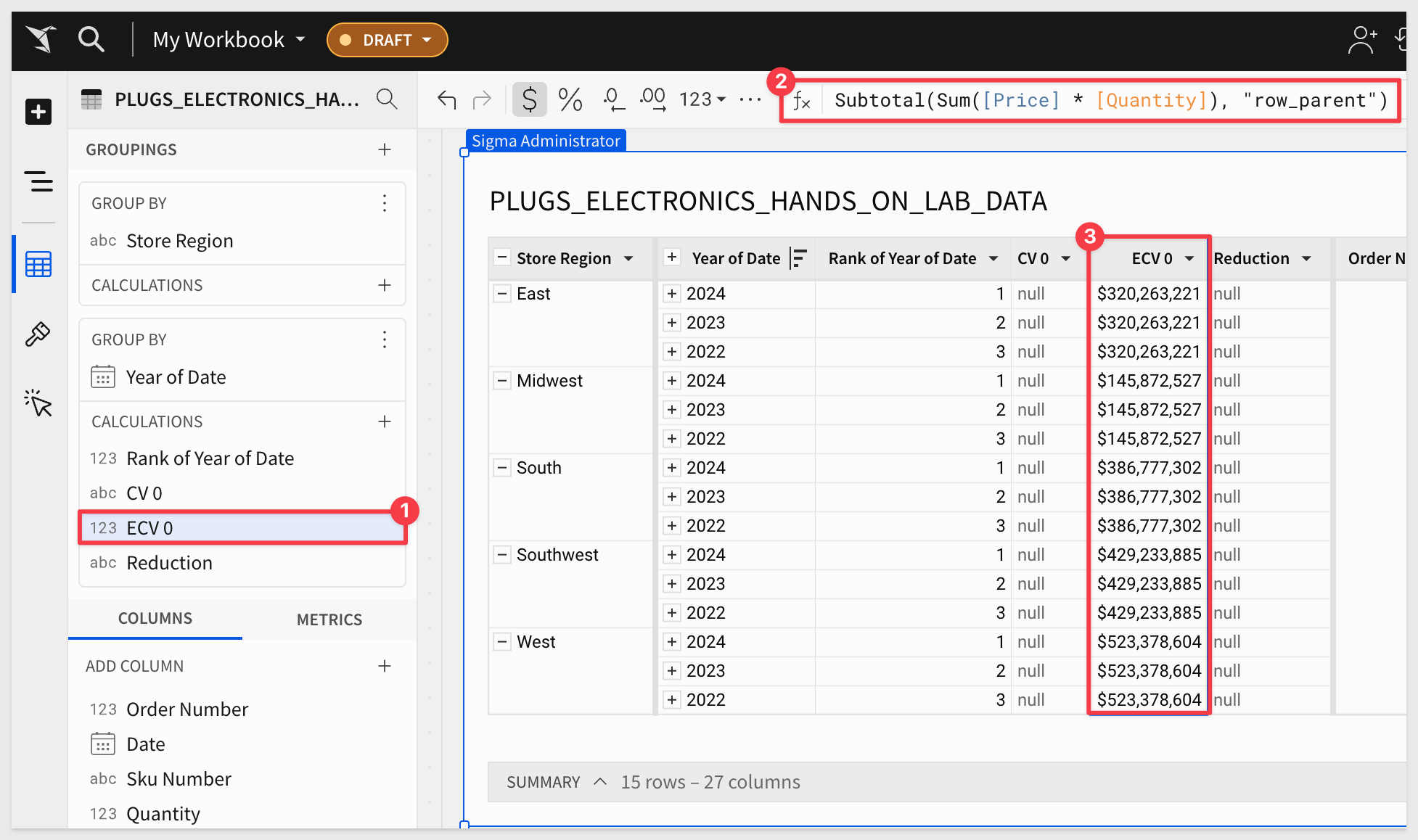
In the ECV 0 column, insert the following formula:
Subtotal(Sum([Price] * [Quantity]), "row_parent")
This calculation will give you the ECV 0 for each Store Region, but keep in mind, this is only accurate for the first year.
The calculation needs to be dynamic, as in year two, we'll introduce a carrying value, which in turn means we'll have a Reduction, resulting in an updated ECV.
Addressing the Recursive Logic
Here is where the challenge arises: the ECV 0 column will inform the CV 0 column, which then informs the Reduction column, and in turn, influences the ECV again.
This cycle moves down row by row for each year, but since Sigma operates on a columnar basis, we need to handle this differently.
We will use helper columns to simulate this recursive logic.
Adjusting the Ending Carry Value
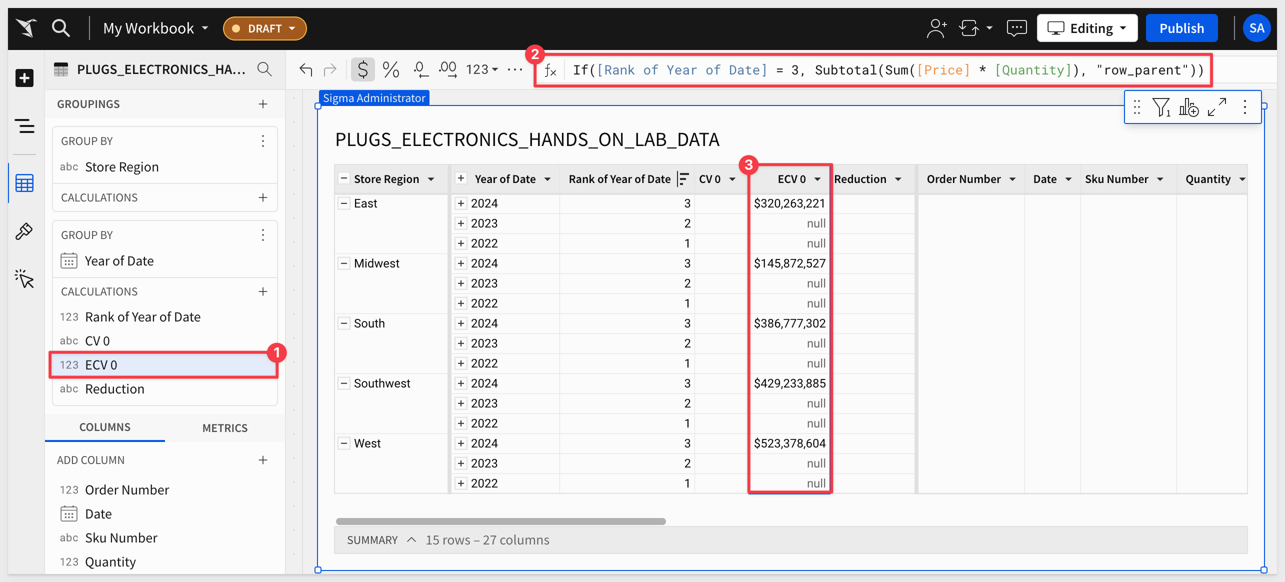
Let's first adjust ECV 0 to ensure it is correctly calculated only for the first year.
Change the formula in ECV 0 to:
If([Rank of Year of Date] = 1, Subtotal(Sum([Price] * [Quantity]), "row_parent"))
This gives us:
Moving the Calculation Forward to Year 2
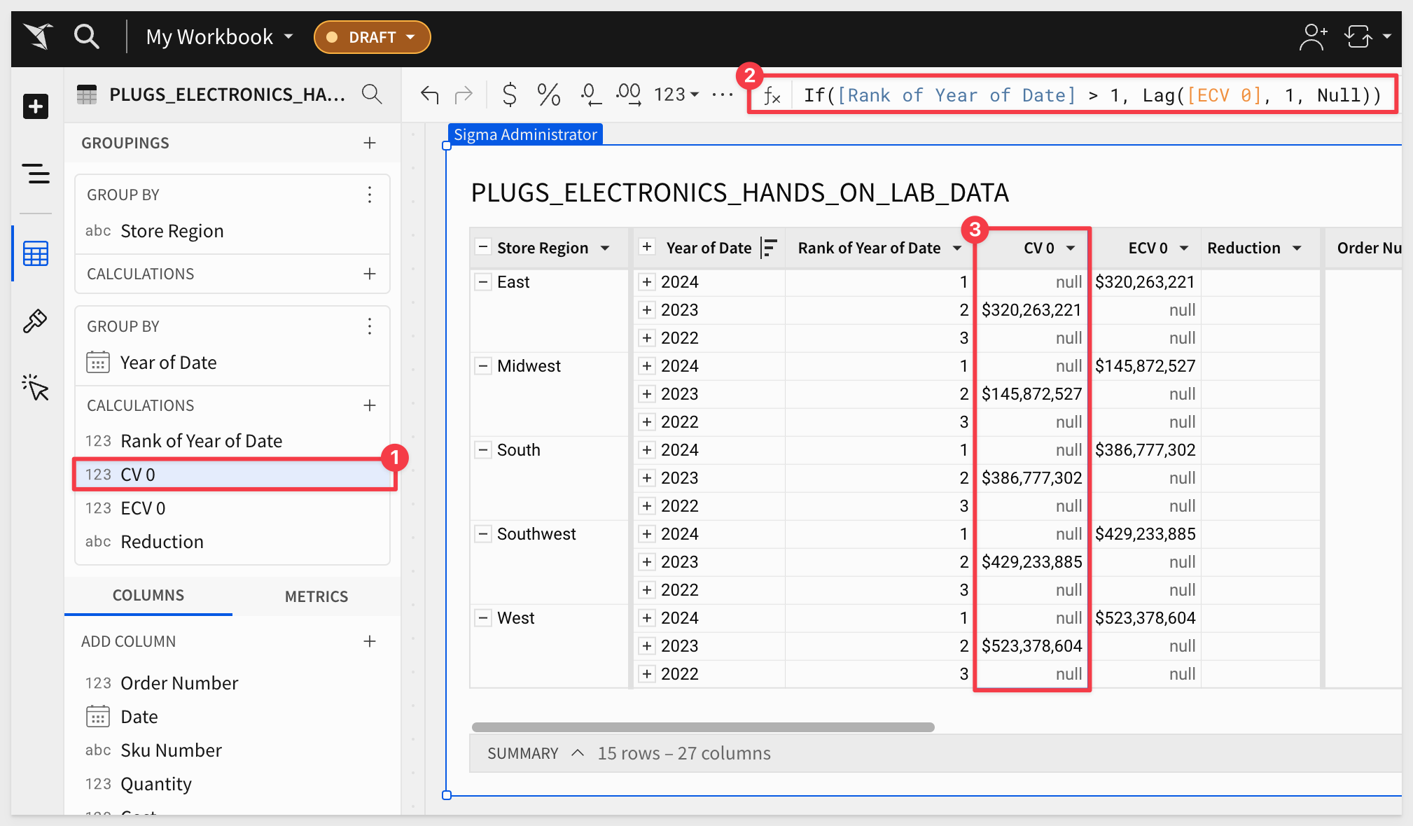
Now, let's transfer this calculation as our carrying value for year two.
In the CV 0 column, insert:
If([Rank of Year of Date] > 1, Lag([ECV 0], 1, Null))
This gives us (after sorting the Year of Date column to show the most recent date first):
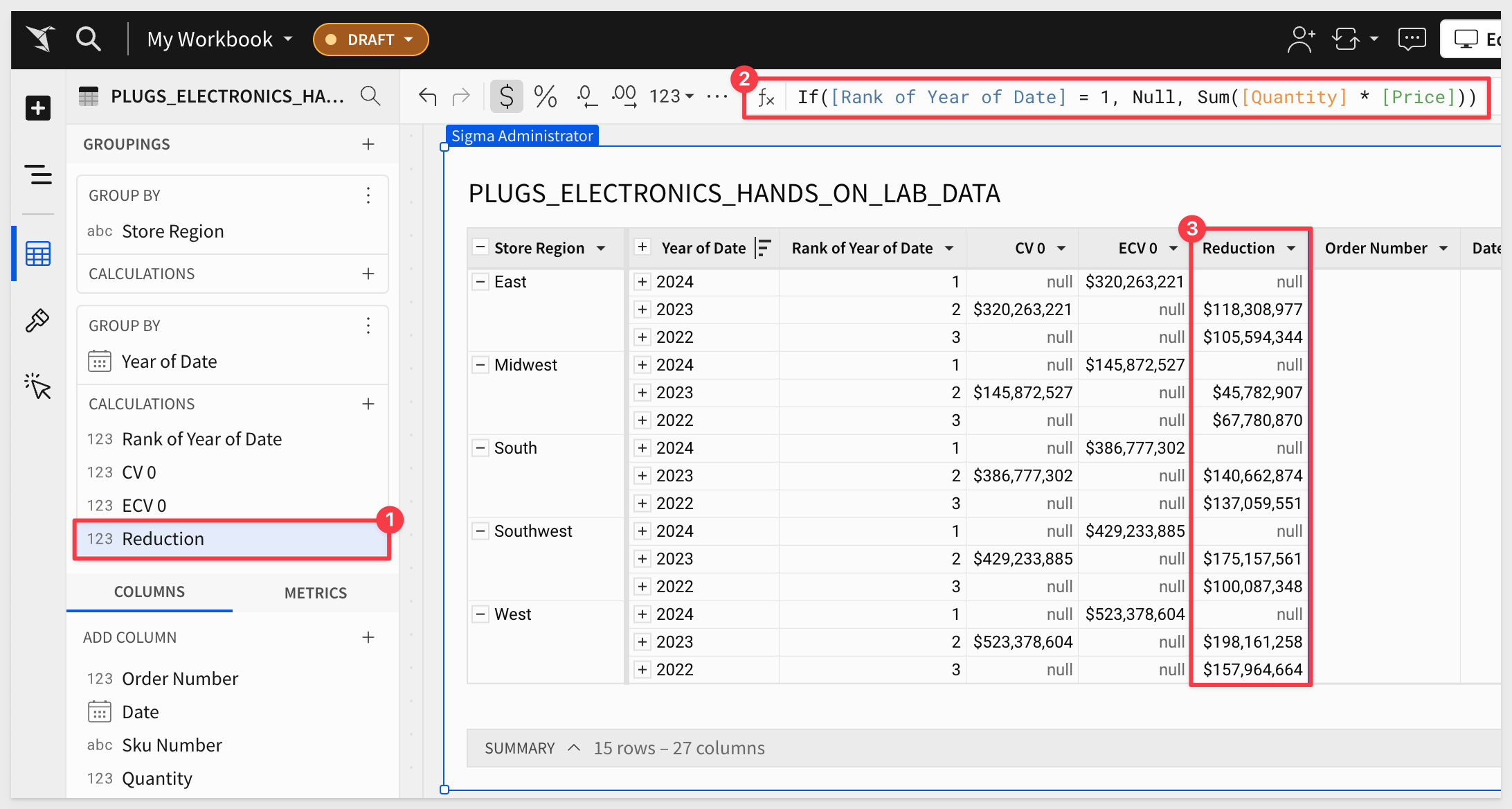
Creating the Reduction Column
Next, define the Reduction column with the following formula:
If([Rank of Year of Date] = 1, Null, Sum([Quantity] * [Price]))
This gives us:
Using Helper Columns for Subsequent Years
Now, we'll create additional helper columns to handle the recursive logic.
Add a new column in CALCULATIONS named CV 1; set its formula to:
If([Rank of Year of Date] = 2, Lag([ECV 0], 1, Null) - [Reduction], Null)
Add a new column named ECV 1; set its formula to:
If([Rank of Year of Date] = 2, [CV 1] - [Reduction], Null)
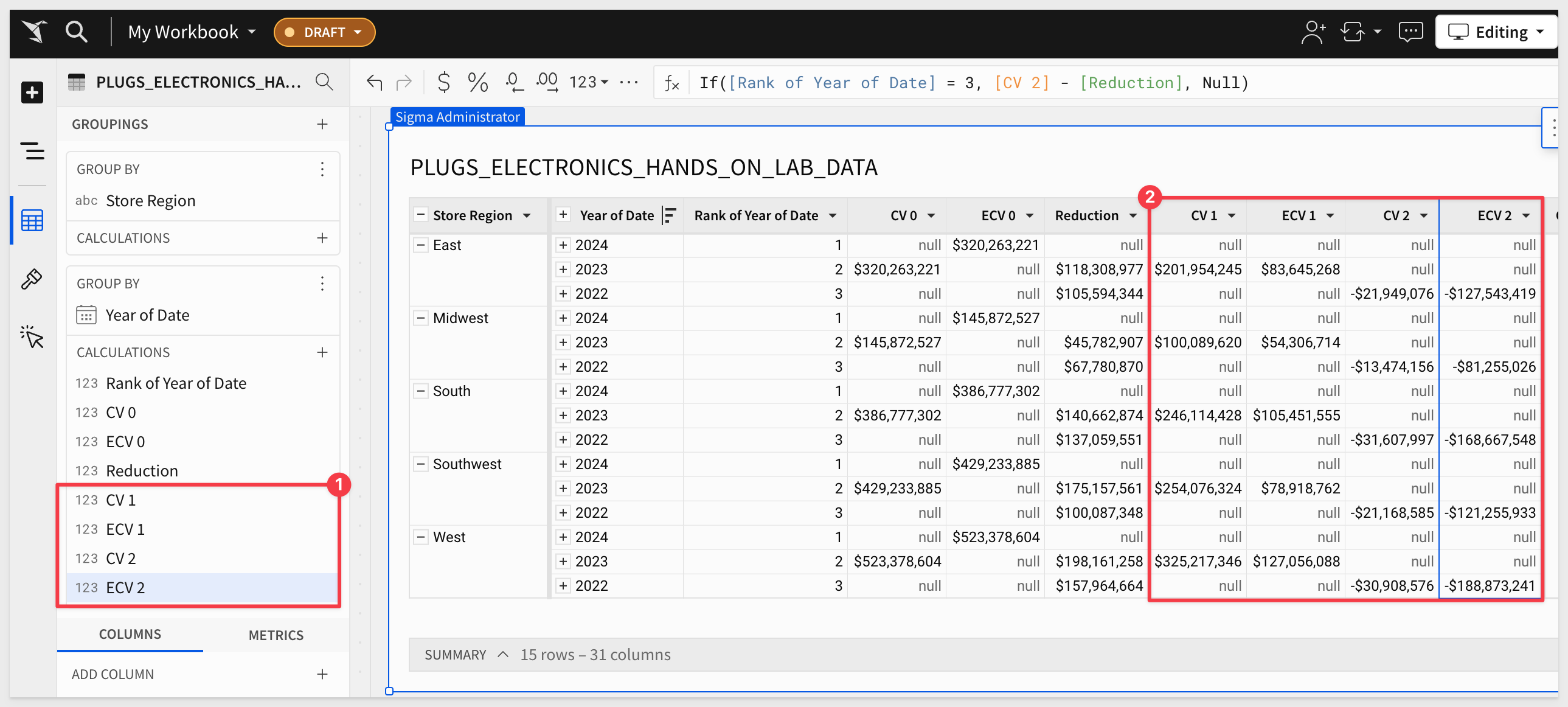
Repeat This Process for Last Year in the Table
Add a new column named CV 2; set its formula to:
If([Rank of Year of Date] = 3, Lag([ECV 1], 1, Null) - [Reduction], Null)
Add a new column named ECV 2; set its formula to:
If([Rank of Year of Date] = 3, [CV 2] - [Reduction], Null)
This gives us:
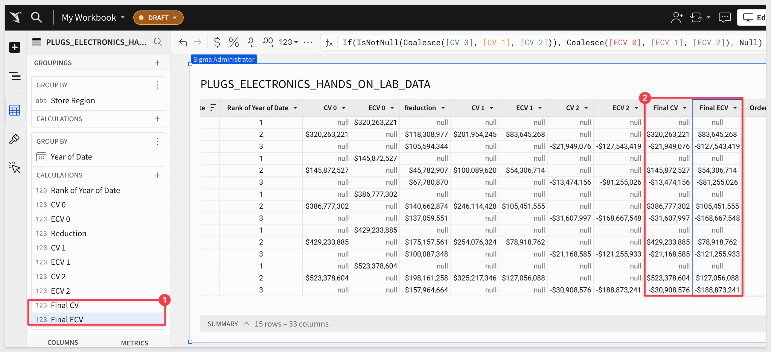
Now that we've created all the necessary columns for carrying values (CV) and ending carry values (ECV) across multiple years, let's consolidate them into a single Final CV and Final EV column to represent the complete discounted cash flow analysis.
Step 1: Create the Final Carrying and Ending Value Columns
Create two new columns in CALCULATIONS and rename them to Final CV and Final ECV.
Use the the following formulas for each:
For Final CV:
Coalesce([CV 0], [CV 1], [CV 2])
This formula will select the first non-null carrying value from the available years. It effectively gathers the carrying value for each row across all years in one column.
For Final ECV:
If(IsNotNull(Coalesce([CV 0], [CV 1], [CV 2])), Coalesce([ECV 0], [ECV 1], [ECV 2]), Null)
Similarly, this formula picks the first non-null ending value from all available EV columns, consolidating them into a single Final ECV column.
This gives us:
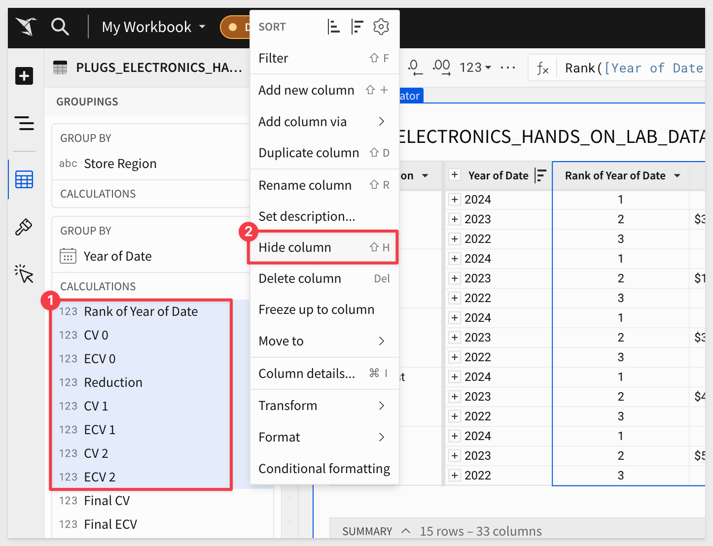
Hide all other CV, ECV and detail columns, now that the values are consolidated into Final CV and Final EV.
This step will make your data cleaner and more user-friendly, ensuring the focus remains on the final results.
Unhide the Reduction column; we want to see that too.
This gives us:
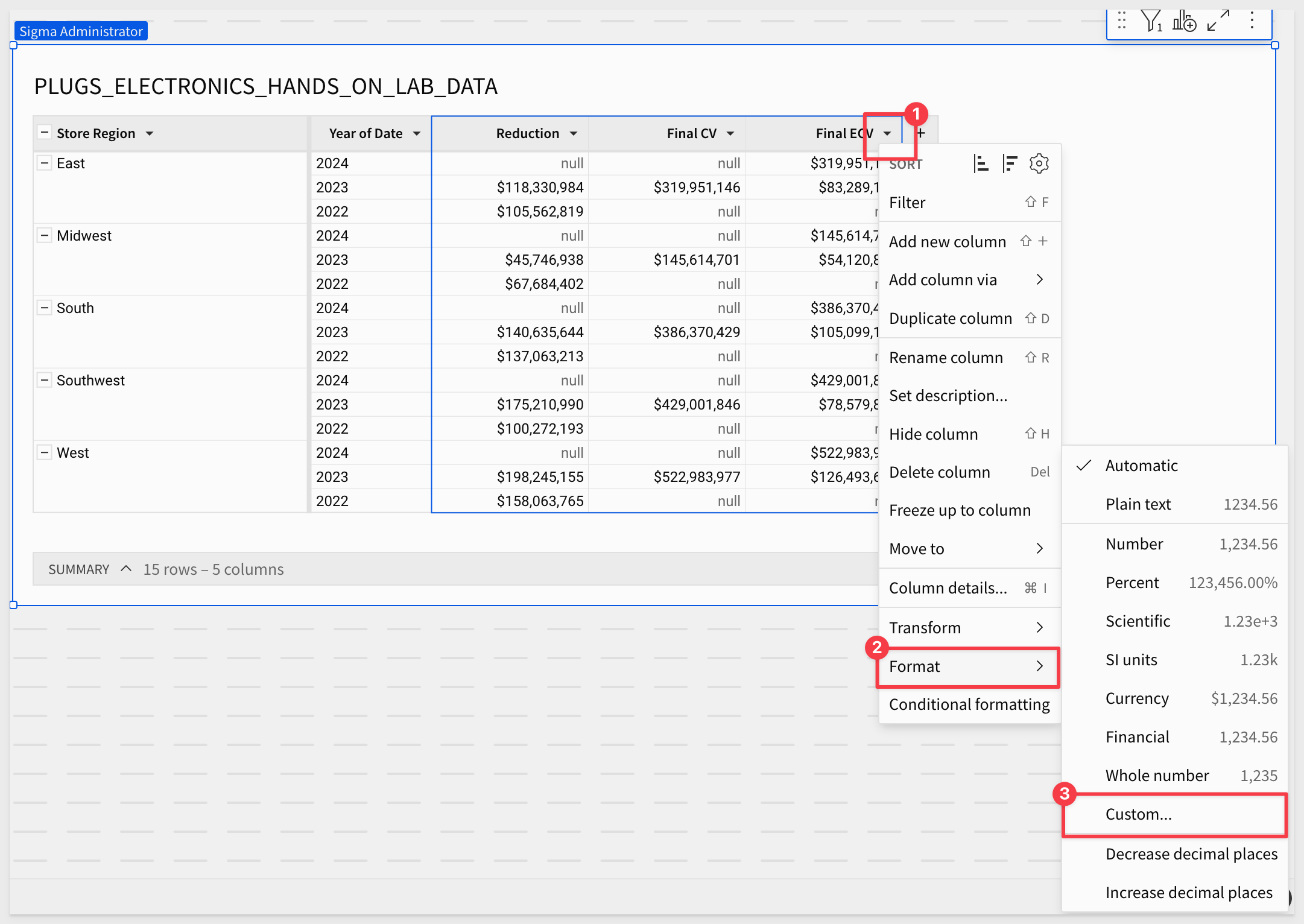
We can also replace the null values with a blank space, to clean up the table more.
Select the Reduction, Final VC and Final ECV columns (shift + click on each column), then open one of the column menus and select Format > Custom:
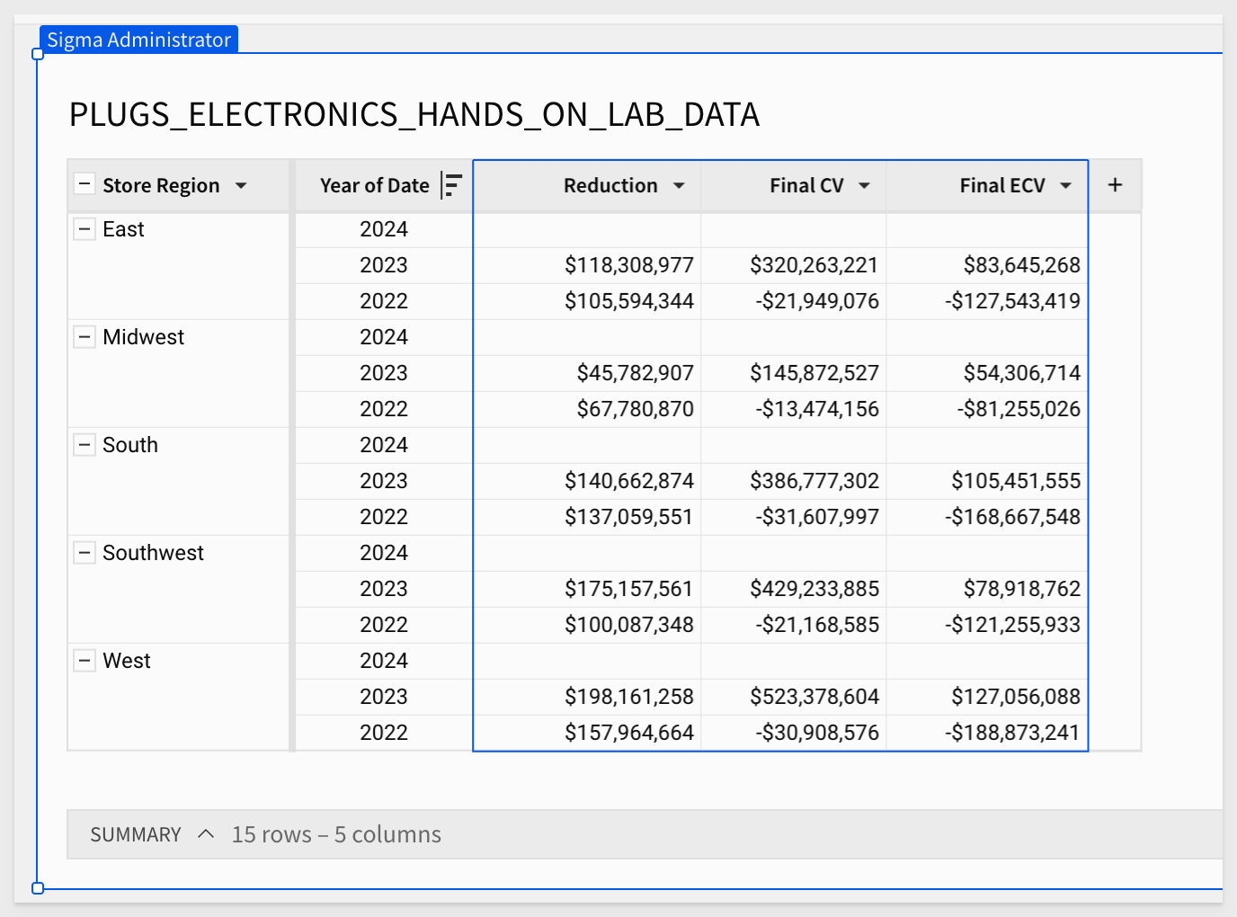
In the Display null as, just add one space (blank text) and click Apply:
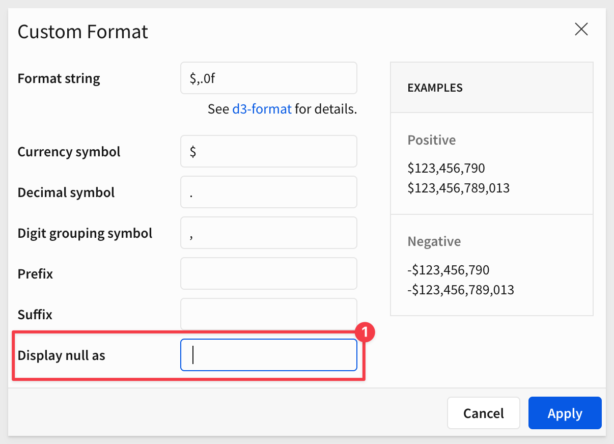
This gives us:
Now we'll calculate the discounted cash flow, which is the ultimate goal of this analysis.
Create a Control Element for the Discount Rate:
Click the + to add a new Control element called at the top of your Sigma workbook.
Rename the control to Discount Rate (WACC)
This control will allow you to input different discount rates interactively, giving you the flexibility to test various scenarios.
Configure the Control
Set the control's configuration as shown.
Enter a percentage value that represents the discount rate (for example: .10). This rate will be applied to your DCF calculations:
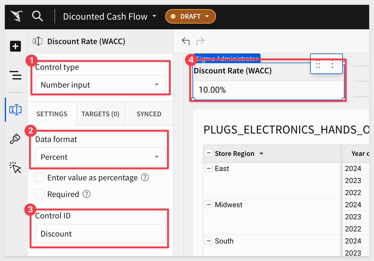
The Discount Rate is used to adjust future cash flows back to their present value. The higher the discount rate, the lower the present value, reflecting the time value of money.
DCF Calculation:
Add a new column in CALCULATIONS and rename this column to DCF.
Enter the following formula into the DCF column:
[Final ECV] / Power((1 + [Discount]), Number([Rank of Year of Date]))
This formula calculates the present value of the future cash flow (Final EV) by applying the discount rate over the specified number of years.
The Power function adjusts the discount rate over the given year, which correctly discounts future values to the present.
The DCF column now represents the value of your asset, project, or investment discounted back to today's terms, using the specified discount rate.
The table now looks like this:
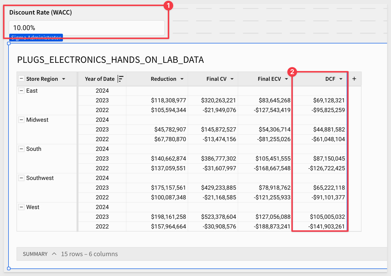
The DCF values now reflect a properly discounted cash flow analysis over time, with larger discounting applied to years further into the future.
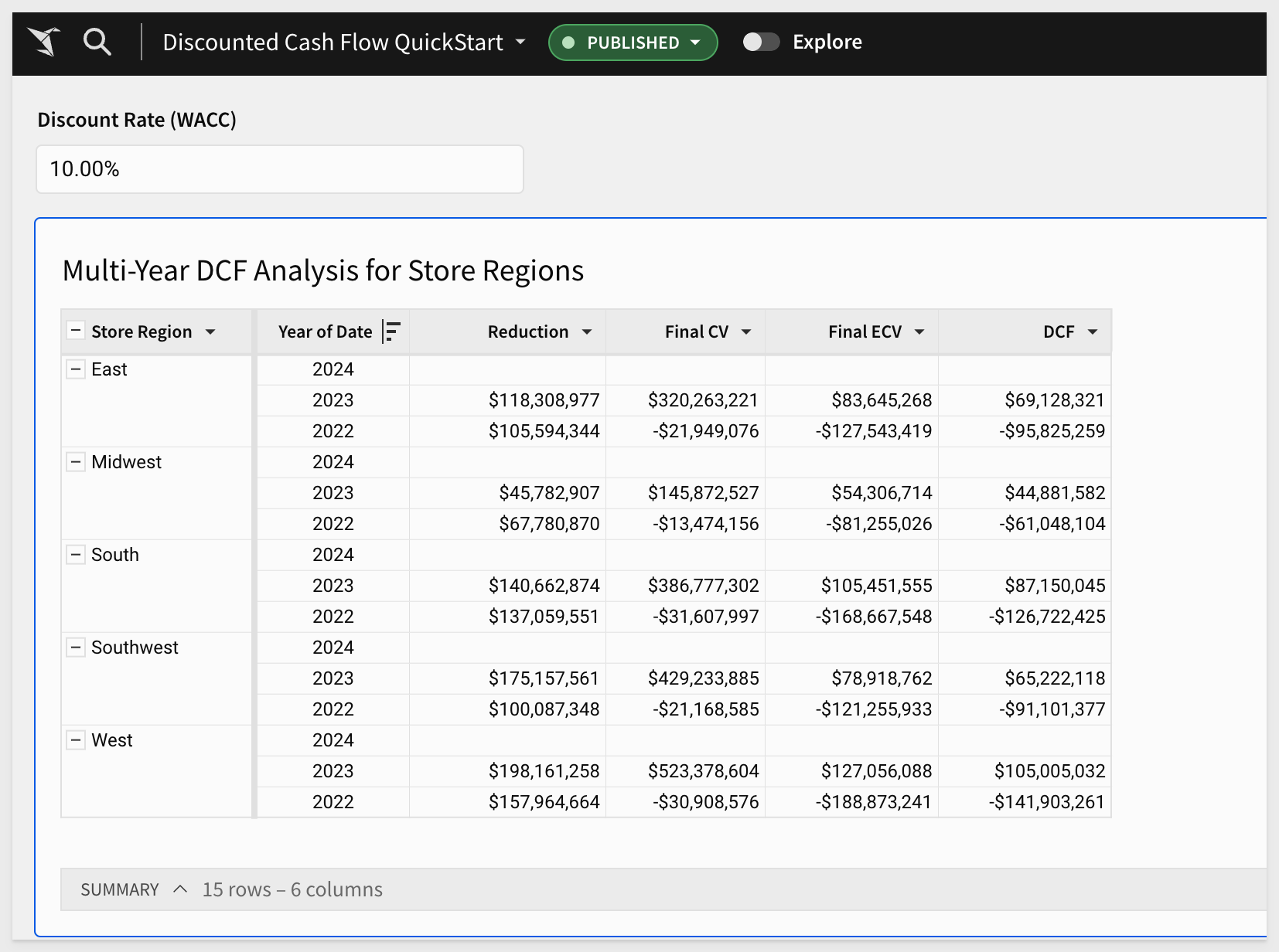
At this point, we should give the table a more appropriate name, so that it is clear to user.
Rename the table to Multi-Year DCF Analysis for Store Regions and Publish the workbook.
Save the workbook as Discounted Cash Flow QuickStart:
In this QuickStart, we covered how to create a discounted cash flow (DCF) in Sigma, using sample data.
Additional Resource Links
Blog
Community
Help Center
QuickStarts
Be sure to check out all the latest developments at Sigma's First Friday Feature page!