Cut query times and reduce warehouse spend by materializing Sigma datasets directly into Snowflake — when to use it, how to configure it, and what to expect from the first run.
For more information on Sigma's product release strategy, see Sigma product releases
If something is not working as you expect, here's how to contact Sigma support
Target Audience
Sigma administrators who are interested in improving performance when working with large amounts of data or just generally interested in learning more about materialization.
Prerequisites
- A computer with a current browser. It does not matter which browser you want to use.
- Access to your Sigma environment.
- Some familiarity with Sigma is assumed. Not all steps will be shown as the basics are assumed to be understood.
- A Snowflake account with the proper administrative and security admin access.
- Write access must be enabled on the Sigma connection to the warehouse.
The concept of storing pre-calculated data for performance optimization (similar to caching) has been around for decades, with many advancements and refinements over time.
Materialization is a form of caching where query results are written into a table in a data warehouse and refreshed at regular intervals (often daily).
This pre-calculated or pre-aggregated data can be accessed more quickly and efficiently than recomputing results every time a query is executed.
This pre-calculated or pre-aggregated data can be accessed more efficiently and quickly than recomputing the results every time the query is executed.
Advantages of Materialization
- Improved query performance: Eliminates repetitive computations, resulting in faster response times.
- Reduced resource consumption: Precomputing and storing results lowers the compute cost of running queries.
- Query optimization: Materialized tables can be indexed or tuned for specific query patterns.
- Enhanced concurrency: Precomputed results allow multiple queries to run simultaneously without contention.
- Simplified data pipelines: Provides a straightforward way to store and reuse intermediate or final query results.

Materialization is a common strategy for improving the performance of interactive queries, but it is most effective in specific situations.
You should consider materializing data when it can provide tangible benefits in query performance, data analysis, or resource management.
At Sigma, we see customers immediately benefit from materialization in use cases such as:
- Flattening complex joins
- Lowering the grain of data (e.g., materializing at an aggregated level)
- Flattening slow calculations (such as JSON extracts)
- Applying a permanent, restrictive filter (e.g., 100M rows exist but only 50K are relevant to the analysis)
Common Use Cases for Materialization
Complex and Resource-Intensive Queries
Queries involving multiple tables, joins, aggregations, or calculations benefit significantly from materialization. By precomputing and storing results, subsequent queries avoid expensive operations and return results faster.
Data Analysis and Reporting
Reporting often involves aggregations, summaries, and transformations. Materializing these results allows analysts to access data instantly, enabling faster insights and smoother reporting workflows.
Time-Dependent Data
For data that changes infrequently or on a predictable schedule, materialization avoids unnecessary recomputation. Materialized tables can be refreshed at regular intervals or triggered by events to balance freshness and efficiency.
Resource Management
Materialization can optimize compute usage by offloading expensive calculations to precomputed tables, freeing live system resources for other workloads.
Matching Grain to Need
If source data contains millions of transactions but reports only need daily, weekly, or monthly summaries, materialization can reduce the data to a smaller, aggregated table. This is often referred to as reducing the grain or reducing cardinality.
Frequently Accessed Data
Data or views accessed repeatedly by many users are good candidates for materialization. By serving queries from precomputed tables, the load on source systems is reduced.
In the software market, there are several options available for caching and materialization, depending on your specific needs and the technology stack you are working with.
Common Options for Materialization
Data Warehousing Solutions (and most RDBMS)
Data warehousing platforms such as Amazon Redshift, Google BigQuery, and Snowflake are designed to handle large-scale analytics workloads. They often provide optimized features for materialization, including materialized views, caching mechanisms, and built-in query optimization techniques to improve performance.
In-Memory Databases
In-memory databases like SAP HANA, Redis, and Apache Ignite store data in memory rather than on disk, which can significantly improve query speed. These platforms often include built-in mechanisms for materialization, such as columnar storage, data replication, and preloading frequently accessed data.
Caching Systems
Caching systems such as Memcached and Redis can be used to materialize frequently accessed data. By storing query results or precomputed data in memory, these systems allow for quick retrieval and reduce repetitive computations.
Custom Data Pipelines and ETL Processes
In some cases, custom materialization solutions may be required using data pipelines or ETL processes. Tools like dbt, Apache Airflow, Apache Spark, or custom scripts can be used to schedule and automate the materialization process, ensuring that materialized data remains up to date.
The availability and specific features of these options will vary depending on the software you choose. It's important to evaluate capabilities, scalability, ease of use, and integration with your existing infrastructure and technology stack before selecting an approach.
With so many available options, deciding where to materialize data can feel complex—but there are some guidelines that can simplify the choice.
Some clients prefer a well-governed, centralized materialization strategy, using a single dedicated tool of their choice. That approach works well in many environments.
In other situations, both approaches can complement each other. For example, some clients use Sigma-based materialization for prototyping and rapid development, since it requires little to no engineering effort and can be done directly by analysts or business teams. Later, once workflows mature, materialization logic can be migrated into the warehouse for long-term production use.
This hybrid approach provides the speed and agility of Sigma during development while ensuring a governed, centralized strategy in production. There are some clear benefits to using Sigma to materialize.
Benefits of Using Sigma to Materialize
- Simple setup in a browser – No special tools required; start materializing in minutes
- No data engineering expertise needed – Enables faster development cycles driven by a broader team
- Role-based access control (RBAC) – Restricts who can materialize data
- Data stays in your cloud data warehouse (CDW) – No new storage systems required
- Automated complexity management – Sigma handles refreshes, dependencies, and orchestration behind the scenes
Governance Considerations
If you choose to use Sigma for materialization, it's important to control who has permission to materialize.
- By default, only Sigma Administrators can materialize.
- You can also create a custom account type (e.g., Creators who can Materialize) and grant that group the materialization permission.
- To avoid uncontrolled growth, it's best to limit this ability to a smaller set of creators, rather than allowing many users to create hundreds of duplicate materializations.
Sigma's RBAC system provides the flexibility to strike the right balance between agility and governance.
Materialization allows you to write workbook elements back to your warehouse as tables, reducing compute costs and improving query performance. By materializing, your data warehouse avoids recomputing the element every time it is used in a Sigma workbook or descendant analysis.
Materializations are stored directly in your warehouse, inside a scratch workspace schema automatically managed by Sigma.
Sigma's query compiler automatically and transparently uses the latest materialization.
All data displayed in Sigma is always queried directly from the warehouse (Snowflake in this case). However, the complexity of the base query carries through to all subsequent queries, including sorting, filtering, and pagination. To solve this, Sigma workbook elements can be materialized back to Snowflake.
This is different from a view object in Snowflake.
In Sigma's implementation, a CREATE TABLE AS statement is used to store the result set of the SQL query generated by the workbook element. You can also materialize a Sigma table that contains multiple grouping levels by selecting a specific grouping level to materialize.
Materializations can be refreshed on a schedule or triggered programmatically via the Sigma API.
By materializing a workbook element, even extremely complex queries can be flattened into a simple SELECT, meaning all downstream queries run with far less strain.
Prepare Snowflake
First, we need to create a database and schema in Snowflake to store our materialized data.
Log in to your Snowflake trial account as ACCOUNTADMIN.
Open a new SQL Worksheet.
Copy/paste the following code:
-- OPERATE AS ADMIN
USE ROLE ACCOUNTADMIN;

-- SELECT WAREHOUSE
USE WAREHOUSE COMPUTE_WH;

-- CREATE DATABASE AND GRANT USAGE
CREATE DATABASE if not exists QUICKSTARTS;
USE DATABASE QUICKSTARTS;
GRANT USAGE ON DATABASE QUICKSTARTS to role sigma_service_account_role;

-- SCHEMA AND GRANT USAGE
CREATE SCHEMA if not exists MATERIALIZATION;
GRANT USAGE, CREATE TABLE, CREATE VIEW, CREATE STAGE ON SCHEMA MATERIALIZATION TO ROLE sigma_service_account_role
Click the dropdown arrow in the upper-right corner and select Run All.
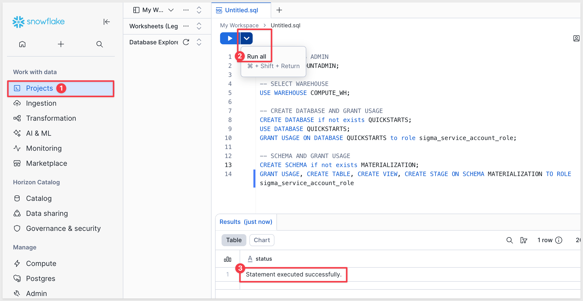
You should see: Statement executed successfully.
Setting up Write Access
Log in to Sigma.
Navigate to Administration > Connections.
Click Create Connection.
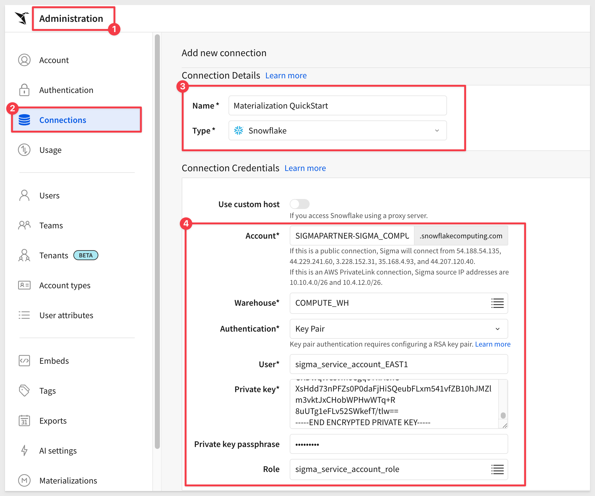
For more information, see the QuickStart Snowflake Key-pair Authorization
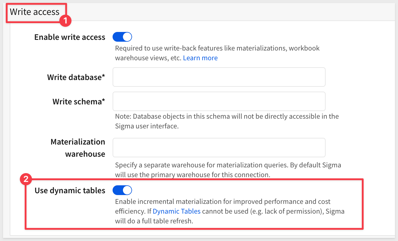
Scroll down to the Write Access section and enter the required information:
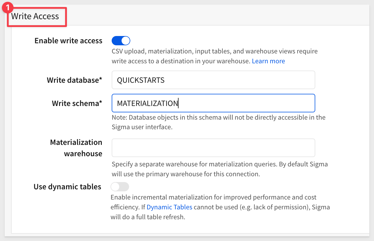 [NOTE: This screenshot may need updating to show the "Enable dynamic tables" option that is now available in connection settings]
Notes on Snowflake Permissions Required for Dynamic Tables
To use dynamic tables in Snowflake, the Snowflake user (or role) connected via Sigma must have the following privileges:
- USAGE on the target database and schema where the dynamic table will be created
- CREATE DYNAMIC TABLE privilege on that schema
- SELECT permission on any underlying tables or views used in the dynamic table query
- USAGE on the warehouse used to run the dynamic table refresh
Additionally, any underlying source tables used in a dynamic table must have change tracking enabled with non-zero time travel retention. Enabling or altering change tracking requires OWNERSHIP of those objects.
Click Create. Sigma will test the connection and, if successful, display a confirmation message.
For more information, see Set up write access
Previously, we discussed materialization in general. Now, let's look at how it is implemented in Sigma at a high level.
What Can Be Materialized
In Sigma, you can materialize any workbook element (table, visualization, pivot) or data model that can be used as a data source for another element.
A materialization is created by scheduling a materialization job. The schedule you choose directly impacts data freshness. Even long-running queries that cannot display in Sigma can still be materialized.
Materializations can be paused (either manually or automatically after a user-specified period of inactivity) and can be deleted at any time.
Advantages of Workbook and Data Model Materialization
- It allows you to materialize any workbook element (table, visualization, pivot) that can be used as a data source for another element.
- Workbook materialization offers a smarter refresh when published. Publishing a document only refreshes the materialization if necessary. For example, if the materialized element hasn't changed, materialization doesn't run. This matters when dealing with very large data, in terms of warehouse cost.
- It offers support for different levels of reference. Grouping levels can be independently materialized.
- Materializations are used when viewing and editing a workbook.
- The workbook viewer is notified of materialization activity in a new "alerts" center (to be integrated with in-app notifications) and toasts.
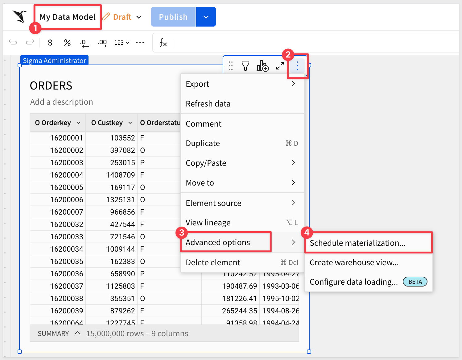
Data models can also be materialized using the same process. Simply access the materialization option from the data model element menu as you would with a standard workbook table:
Limitations
Parameters and system functions:
Materialization is not available for data that use parameters or most system functions, with a few exceptions. For example, the system function Today() does work.
Data is expected to return different values when parameters change. Materialized tables, however, always return the same fixed output generated at the time the materialization ran. Using them with parameterized elements could produce unexpected results.
Row-level security:
Materialization is incompatible with row-level security. If user-attribute functions are referenced, the materialization will error.
Data referencing other data:
Data that duplicates or joins other data can usually be materialized. However, if any underlying data cannot be materialized, the dependent data cannot be either.
Dependent Materializations
When one materialized element references another (for example, a workbook table built on top of another materialized workbook element), Sigma automatically manages the refresh order to ensure data consistency.
This makes it simple to build multi-layered data pipelines where aggregated tables build on detailed materializations, while maintaining data consistency across all layers.
For this exercise, we'll use the Snowflake sample database TPCH_SF10, which contains an ORDERS table with 9 columns and ~15M rows.
Typically, materialization in Sigma is applied after joining tables, adding groupings, and creating calculated columns. As discussed earlier, flat tables by themselves won't benefit much from materialization.
For simplicity, we'll assume that some joins and calculated columns already exist, but we'll skip that setup here so we can focus directly on how to materialize data in Sigma. A more complex, grouped example will follow later.
In Sigma, click the  icon to return home.
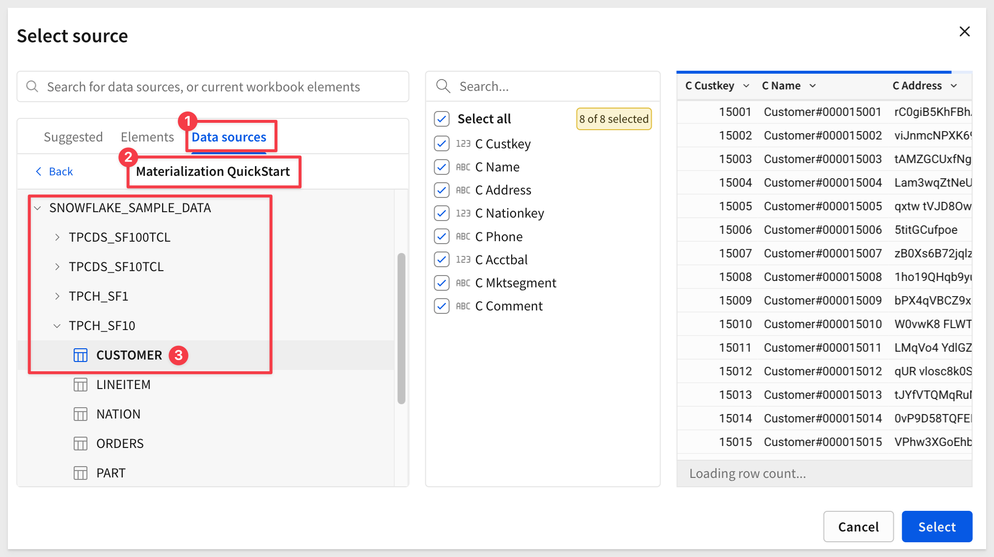
Select Materialization QuickStart from the left side-bar:
Expand the database SNOWFLAKE_SAMPLE_DATA > TPCH_SF10 and select the ORDERS table. Click Explore:
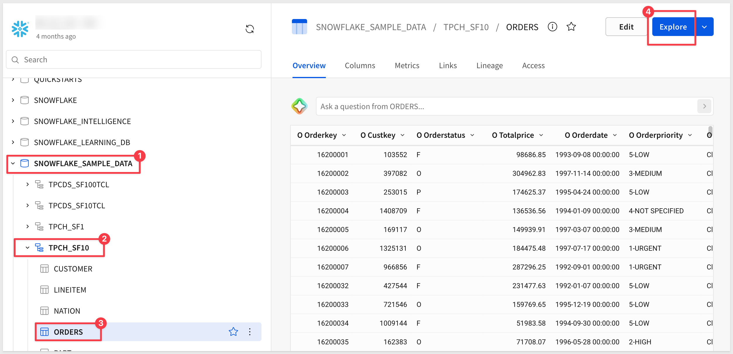
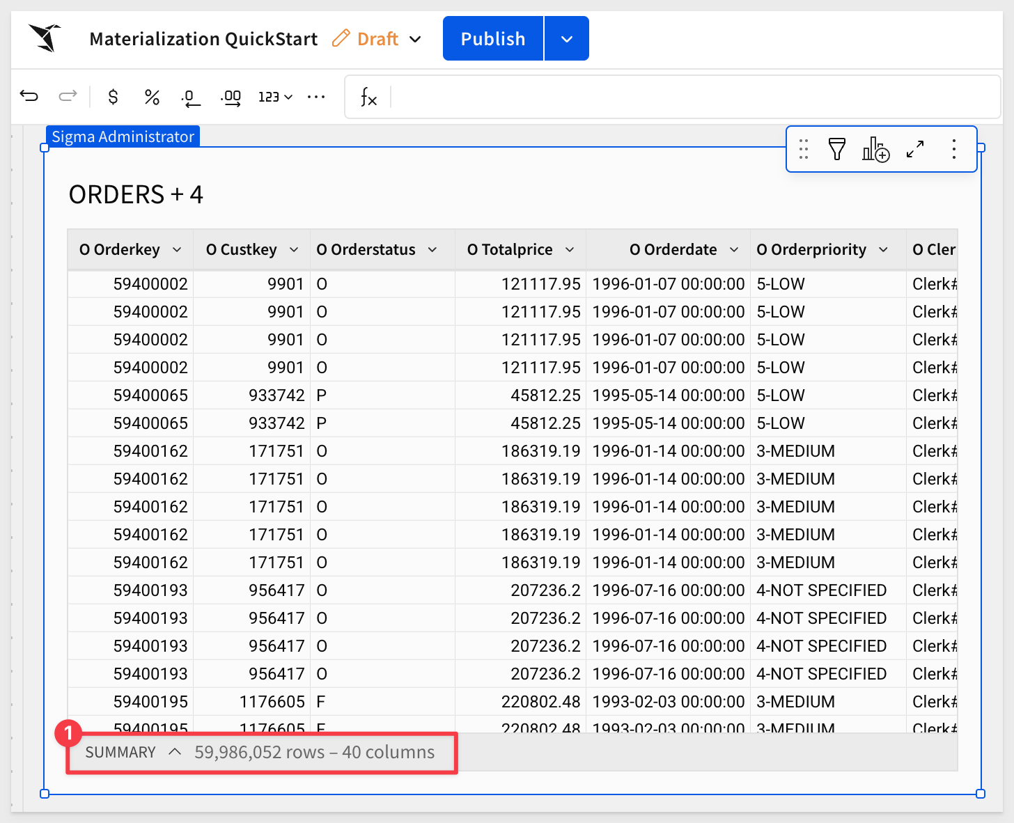
The Orders table opens in an unsaved workbook. All 9 columns are selected, with 15M rows available:
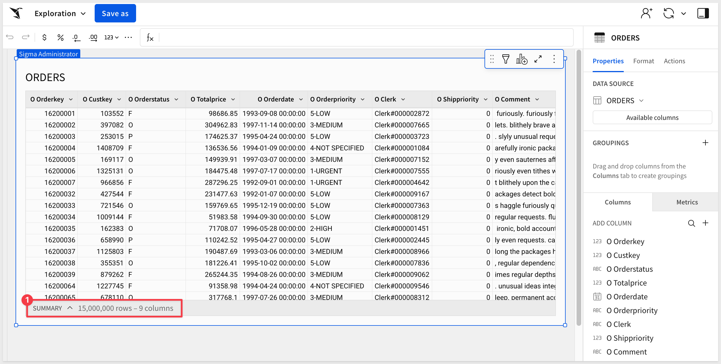
Save this workbook as Materialization QuickStart.
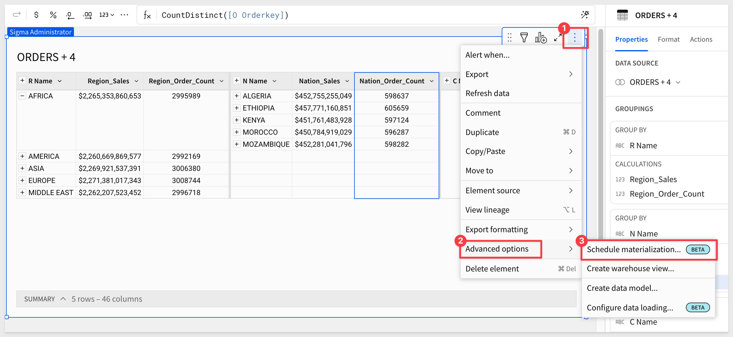
Click the hamburger menu (3 dots) and select Advanced options > Schedule materialization:
In the Materialization schedules modal, create a new schedule.
Since the workbook only contains one element (Page 1 – Orders), that element is pre-selected.
Set the schedule to run once daily at 3:00 AM in your local timezone.
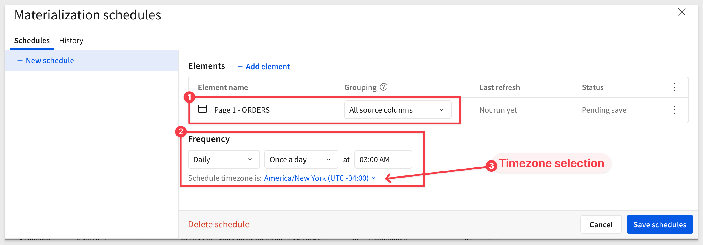
Click Save Schedules.
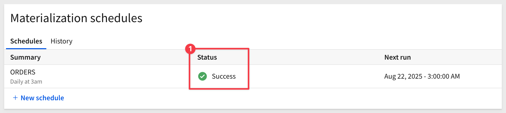
The materialization will run immediately, with a status of Pending > In progress and finally Success:
The UI will display the next scheduled run time:
Close the schedule window.
Navigate back to Administration > Materializations where we can see the list of our current jobs:
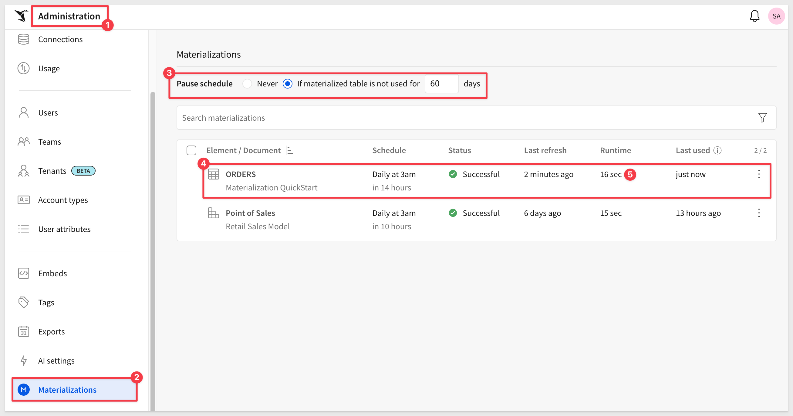
Here you can check the last run status, duration, and row count. In this example, the job processed 15M rows in 16 seconds using a Snowflake X-Small warehouse.
Click on the Orders text to return to the Materialization QuickStart workbook.
Click the View materialization icon to see:
- Details about the most recent run
- A Materialize now button
- Links to View Schedule pages
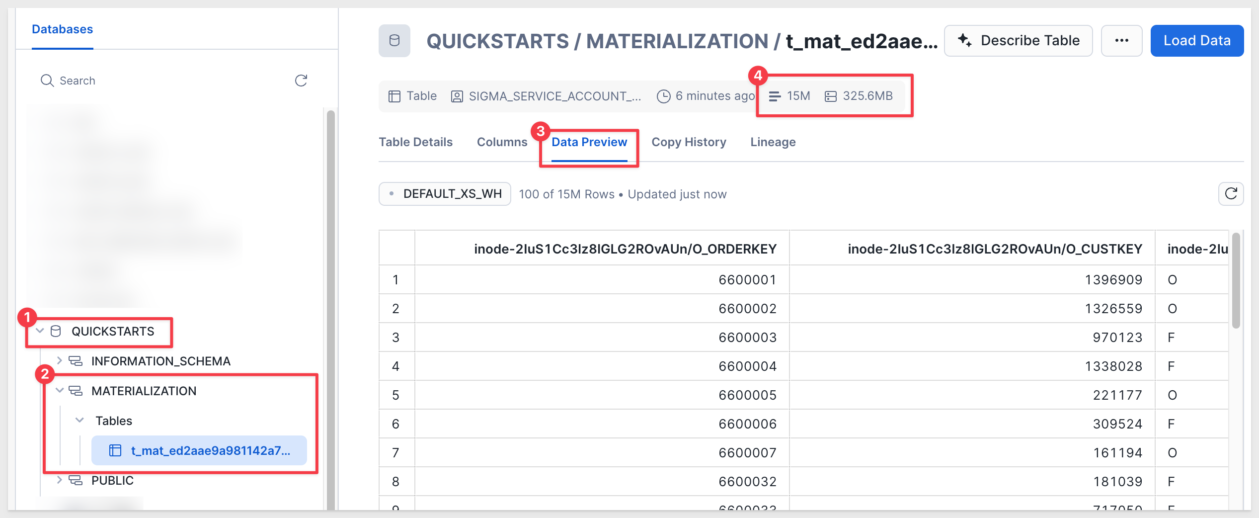
Sigma creates a new table in Snowflake based on your materialization configuration (in this case, 15M rows).
The table is stored in a scratch schema that Sigma manages automatically. While the column data may not appear in a user-friendly format, this schema is fully transparent to Sigma users and is not intended for direct use.
Materialization improves query performance by allowing your data warehouse to reuse precomputed results instead of recomputing the element each time it is used in a Sigma workbook or descendant analysis.
If you need to access this data from other applications, see Review warehouse view details
Dynamic tables in Snowflake enable incremental refresh for materializations. Instead of rebuilding the entire materialized table on each refresh, Sigma only updates the rows that have changed since the last run.
This represents a significant enhancement to materialization capabilities.
Key Benefits:
- Reduced compute costs - Only changed data is processed
- Faster refresh times - Smaller updates complete quicker
- Automatic optimization - Sigma skips scheduled runs when no data has changed
- Same user experience - Works transparently in the background
How It Works
When you configure a Snowflake connection to use dynamic tables:
- Sigma creates a Snowflake dynamic table instead of a regular table
- Snowflake's change tracking monitors the source data
- On each scheduled run, only modified rows are updated
- If no changes occurred, the run is automatically skipped
Requirements for Dynamic Tables
To use dynamic tables with materialization:
Connection Configuration:
- Your Snowflake connection must be configured to use dynamic tables
- This is enabled in
Administration>Connections>Edit your connection:
Source Table Requirements:
- Change tracking must be enabled on source tables in Snowflake
- Tables must have non-zero time travel retention
- You need
OWNERSHIPprivileges to enable change tracking
Supported Elements:
- Workbook elements (tables, visualizations, pivots)
- Data model elements
When to Use Dynamic Tables
Dynamic tables are ideal when:
- Source data changes incrementally (new rows added, updates to existing rows)
- Materialized tables are large (millions of rows)
- Refresh frequency is high (hourly or more frequent)
- Compute cost optimization is a priority
Example scenarios:
- Order tables with new transactions added daily
- Customer tables with periodic attribute updates
- Event logs with streaming data ingestion
- Sales data with regular incremental loads
For more information, see Incremental materialization with dynamic tables
Aggregate navigation is an advanced BI design approach where we create several materialized tables of different grain behind the scenes, then seamlessly swap the data sources between these tables as the user changes their grain of analysis. The benefit is fast performance at higher levels of aggregation, combined with the depth of analysis at lower levels — all transparent to the end-user.
Using conventional BI tools, aggregate navigation can be costly to implement, since you often need to manually create and populate several aggregated tables, then add complex logic to auto-navigate between them.
By contrast, aggregate navigation in Sigma is straightforward.
Aggregation functions or operators are applied to groups of data to calculate consolidated values. Some common functions include sum, count, average, minimum, maximum, and median. These can be applied to numerical data (e.g., sales figures, temperature readings) as well as categorical data (e.g., the number of occurrences by category).
Aggregations are widely used to generate reports, analyze trends, or derive meaningful statistics from data. For example, in a sales database, you might calculate total sales by product category, average revenue per customer, or the highest-selling region.
Aggregations can be applied at different levels — entire data collections, specific groups or categories, or across multiple dimensions. The choice depends on analysis goals and data structure.
Tables that leverage aggregate navigation are excellent candidates for materialization.
In this section, we'll demonstrate building a table that joins four other tables and contains ~60M rows. You can follow along, though performance may be slower in trial accounts using an X-Small Snowflake warehouse.
Some general rules:
- Any materialization with multiple levels creates tables for the selected level and each level above it.
- If you have four groupings plus a base level, aggregating "all columns" will materialize five tables total.
- All visualizations have at least one grouping level.
- If you want to materialize only a single aggregated grouping level, you can create a child table and materialize that.
- Materializing all grouping levels allows you to build aggregation tables that downstream elements can reference efficiently.
For example: If we have five grouping levels in a table element and materialize at the third level, Sigma creates three materializations: one for the top level, one for the second level, and one for the third. The fourth, fifth, and base grouping levels will not be materialized.
This trade-off matters: performance vs. storage cost. If levels four and five contain hundreds of millions of records, Sigma still allows materialization of levels one through three — delivering strong performance with the option to drill deeper when needed (though more slowly).
We'll build on the existing workbook but extend the data.
Sample Use Case
Users viewing Sigma content often want to see sales data rolled up from the Region/Nation/Customer level, with summary sales totals and order counts broken out for each group. They rarely explore line item detail but want the option to do so occasionally.
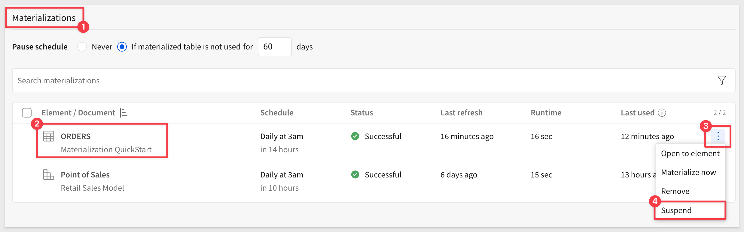
First, pause the existing materialization schedule so it no longer runs.
You can do this either in the workbook or in Administration > Materialization:
The ORDERS schedule status will switch to Suspended.
Click Orders to return to the workbook and then click Edit.
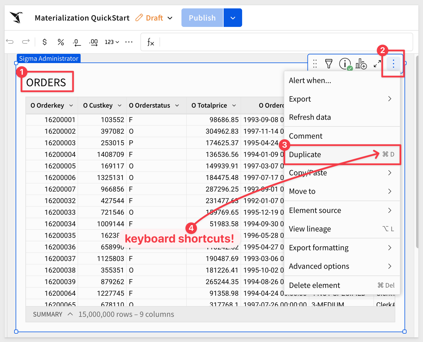
Now, make a duplicate of the Orders table:
Move the duplicate to a new page:
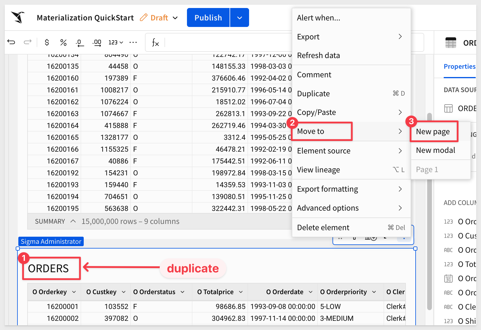
You can also copy/paste the table instead.
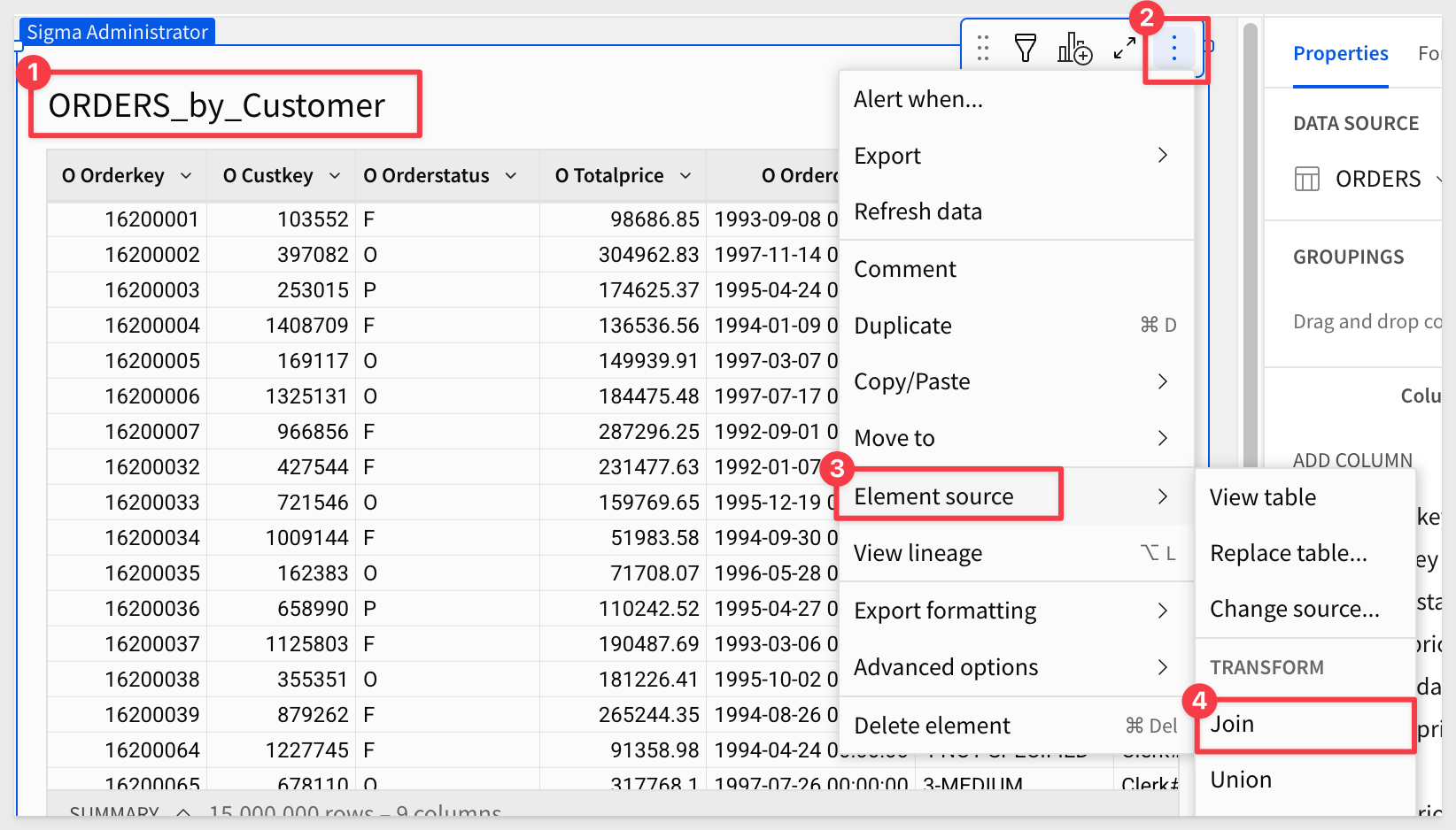
Rename the new table ORDERS_by_Customer.
Join tables
Next, we'll join the CUSTOMER table (from the database) to ORDERS.
Click Join:
Navigate the UI to locate theMaterialization QuickStart connection, expand the tree, and select TPCH_SF10 > CUSTOMER. Click Select.
Set the join keys: O Custkey = C Custkey.
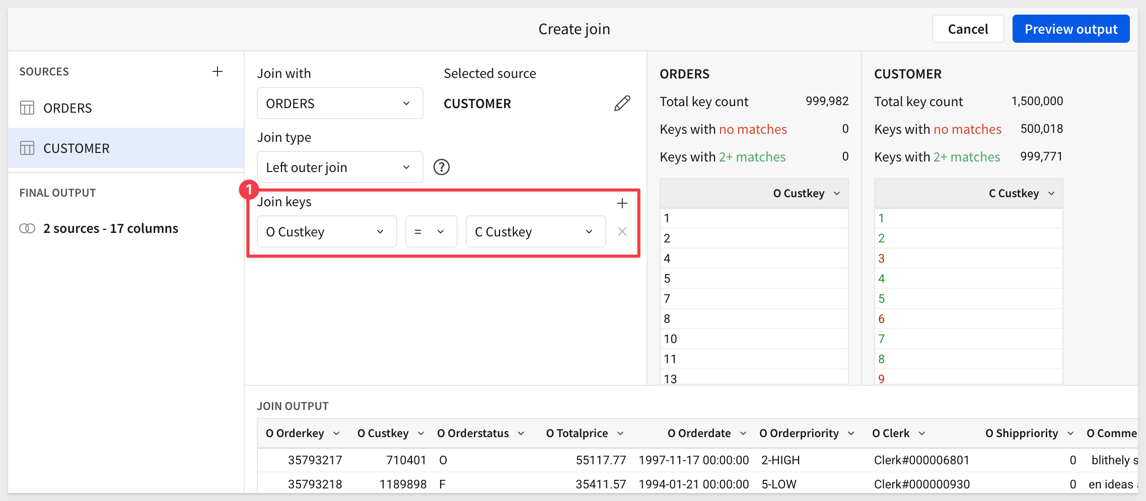
The result will show some customers with no orders and some with multiple.
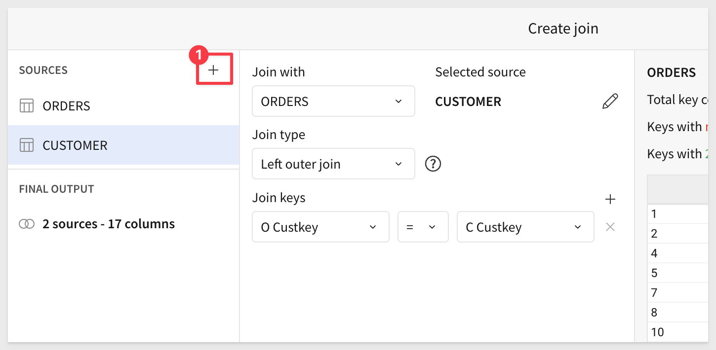
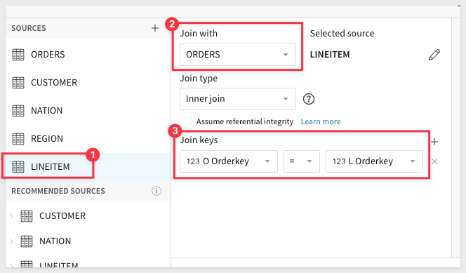
Click the + icon to add another join:
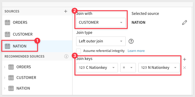
Repeat the process to join the Nation table to the Customer table (not Orders):
Join the Region table to the Nation table:

Join the Line Item table to Orders:
Click Preview Output.
Sigma displays the lineage, which shows a visual representation of how the data is mapped.
Looking at the lineage, we'll materialize at the Region level and treat the LineItem level as our "base" or less frequently used data that we won't materialize.
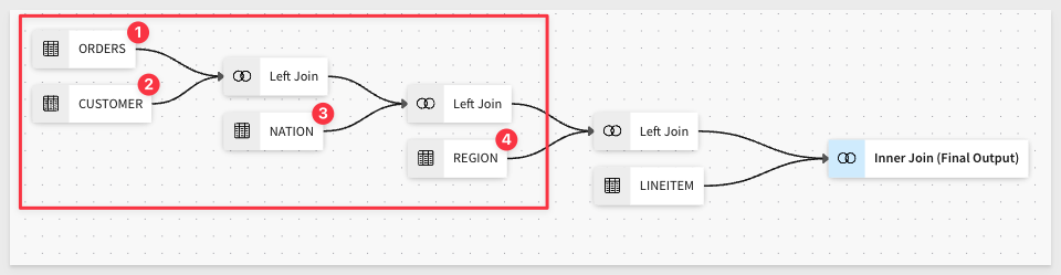
Click Done.
We now have about 60M rows of order detail by customer:
Add calculated columns
Add new columns, naming and setting each formula as shown below:
NAME: FORMULA: (note: they are all the same, using the groupings)
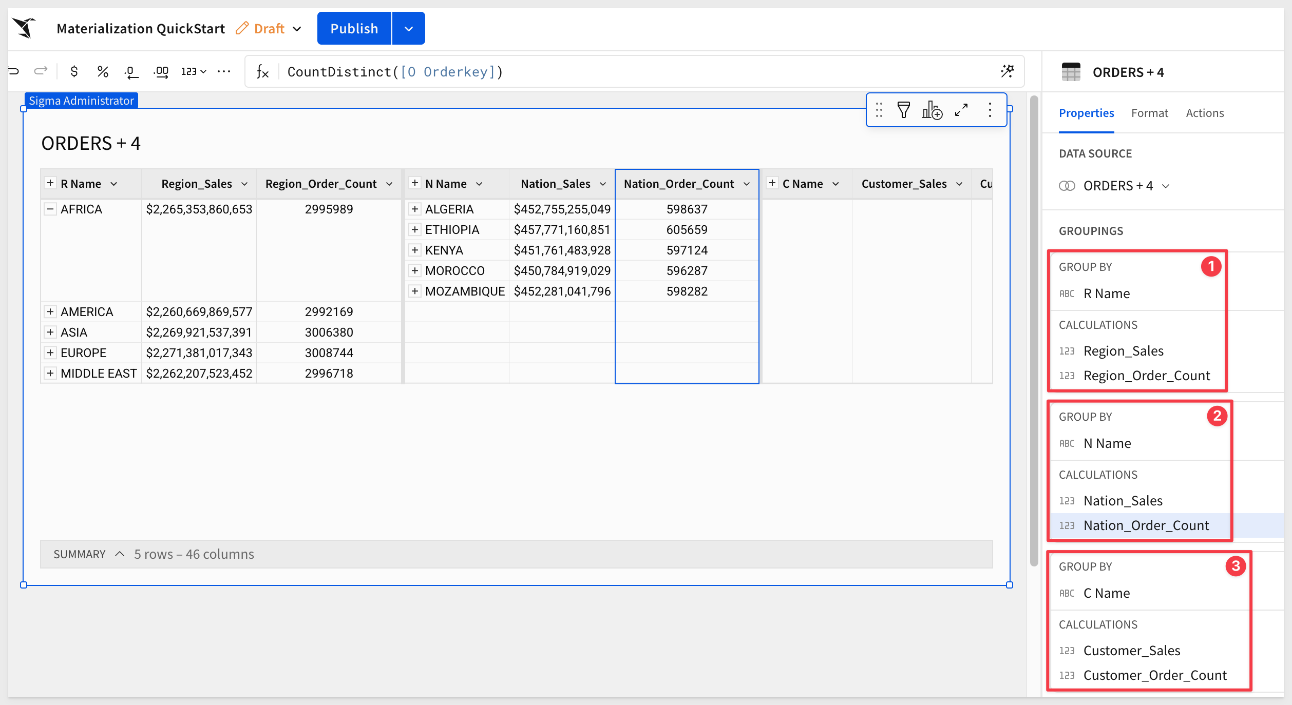
Region_Sales Sum([O Totalprice])
Region_Order_Count CountDistinct([O Orderkey])
Nation_Sales Sum([O Totalprice])
Nation_Order_Count CountDistinct([O Orderkey])
Customer_Sales Sum([O Totalprice])
Customer_Order_Count CountDistinct([O Orderkey])
Data grouping
Create the following three groups in Sigma:
Be sure to click Publish when done.
Materialize
Now that the table is ready, we can materialize again — this time with the option to select a grouping level.
Open the Schedule materialization UI:
Create a schedule (once per day) based on the Customer grouping level:
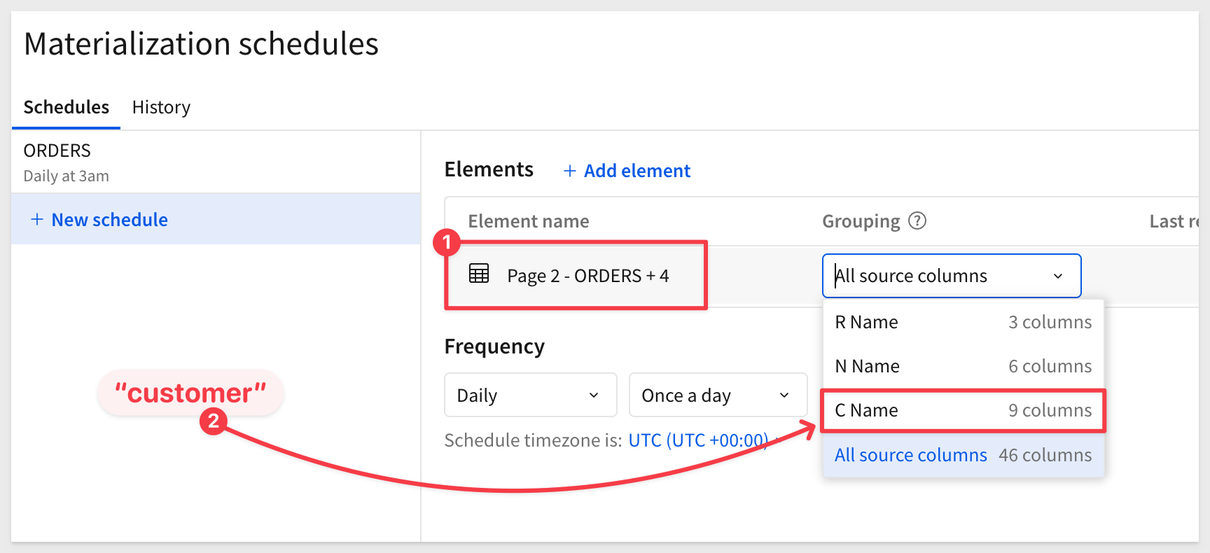
Once complete, three new tables will appear in Snowflake.
Looking at the Sigma WriteDB, the three tables are organized with the lowest level first, followed by the next two grouping levels. Column names are not "friendly" — this is intentional:
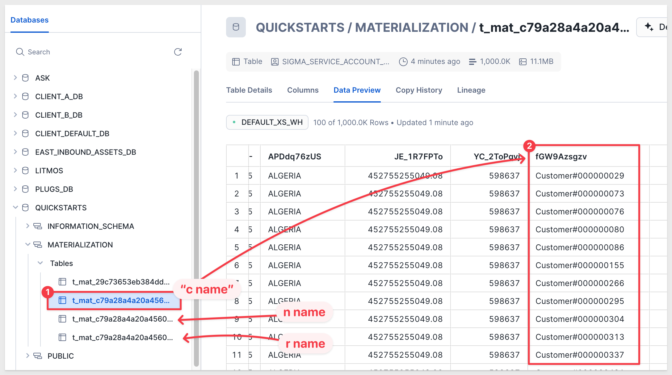
It is possible to access this data from other applications using Sigma's Warehouse Views feature.
Once materialized tables are accessed, they also exist in the warehouse cache (subject to Snowflake caching rules), further improving performance.
For those interested, please refer to the Sigma on Snowflake Best Practices guide
This QuickStart was designed as a primer on materialization and the questions and considerations that surround it.
We defined what materialization is, provided guidance on when and why to use it, and discussed who typically sets it up.
Finally, we stepped through using Sigma and Snowflake to materialize data — including examples with grouped data.
Additional Resource Links
Be sure to check out all the latest developments at Sigma's First Friday Feature page!
Help Center Home
Sigma Community
Sigma Blog