This QuickStart covers some of the more common questions we receive from Sigma customers. It is not comprehensive but is intended to present topics that often arise after users have completed the QuickStart Fundamentals and begin using Sigma with their own data.
We are happy to get feedback and suggestions on other topics for QuickStart that may be of interest to you.
If you have comments, please feel free to open an issue here.
For more information on Sigma's product release strategy, see Sigma product releases.
Target Audience
Sigma users who have recently completed the QuickStart Fundamentals or have some experience using Sigma in general.
Prerequisites
- A computer with a current browser. It does not matter which browser you want to use.
- Access to your Sigma environment.
- Some familiarity with Sigma is assumed. Not all steps will be shown as the basics are assumed to be understood.

Sigma makes data modeling really user-friendly, as we will demonstrate in this section using our sample data.
Log into Sigma and create a new workbook.
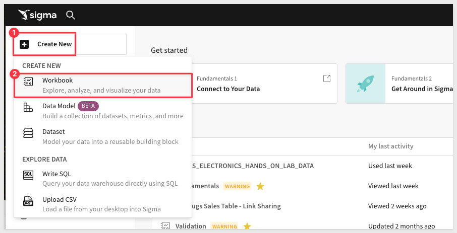
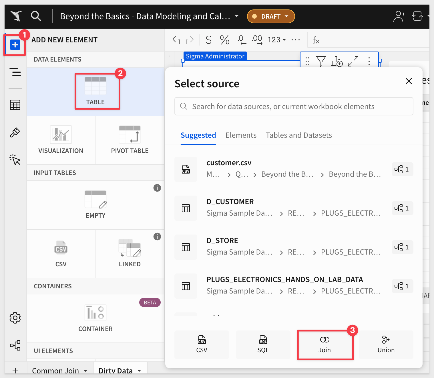
Select TABLE > JOIN:
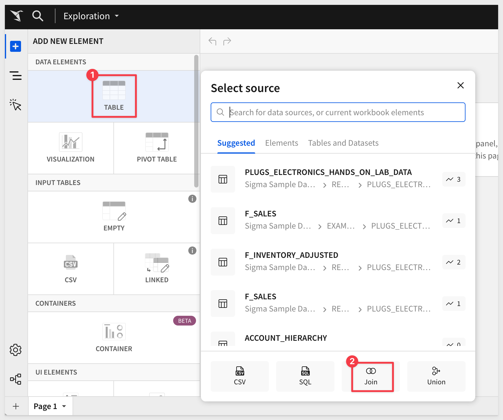
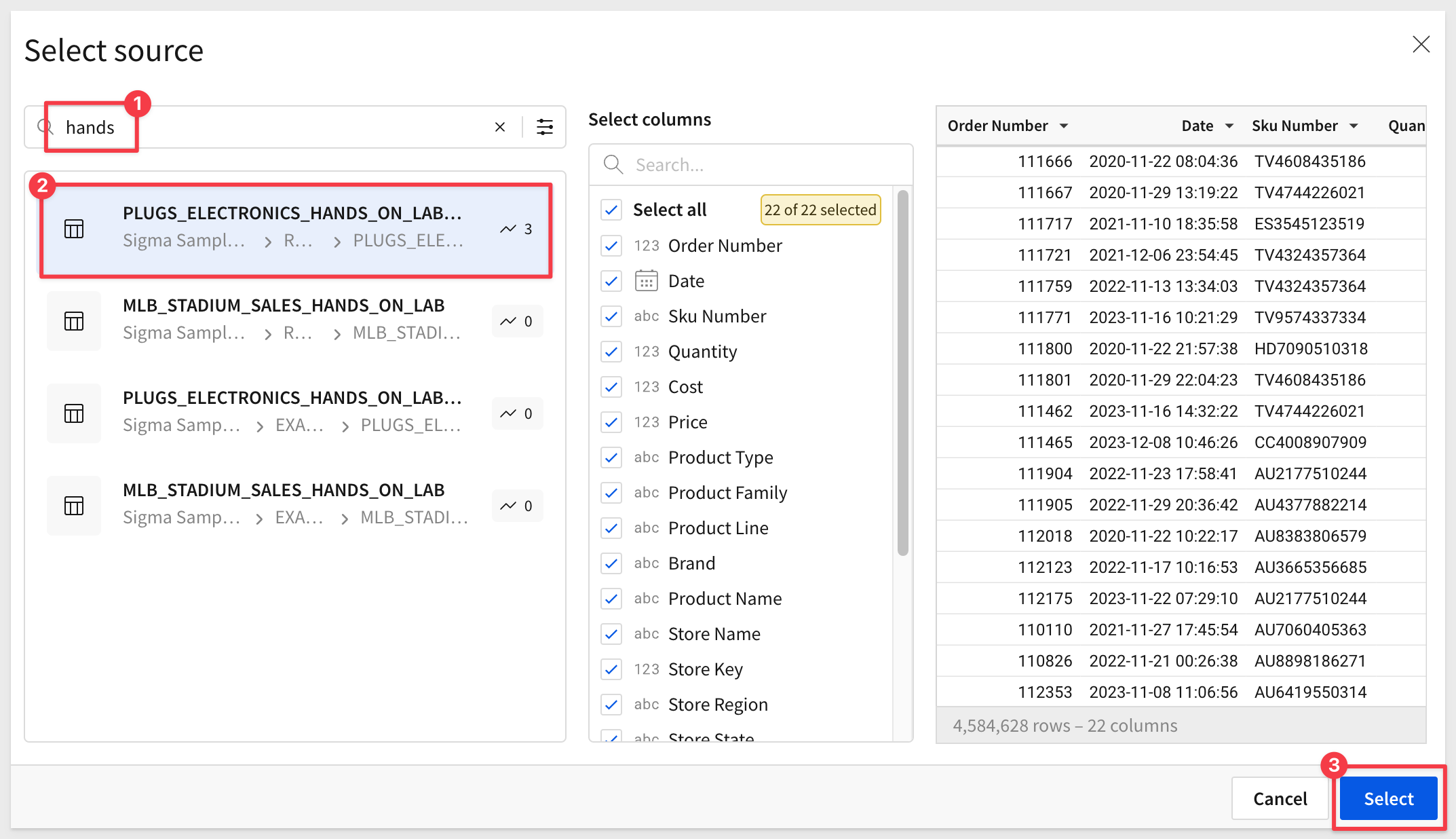
In the search bar, enter Hands and select the PLUGS_ELECTRONICS_HANDS_ON_LAB_DATA table. For now we will accept all columns.
Click Select:
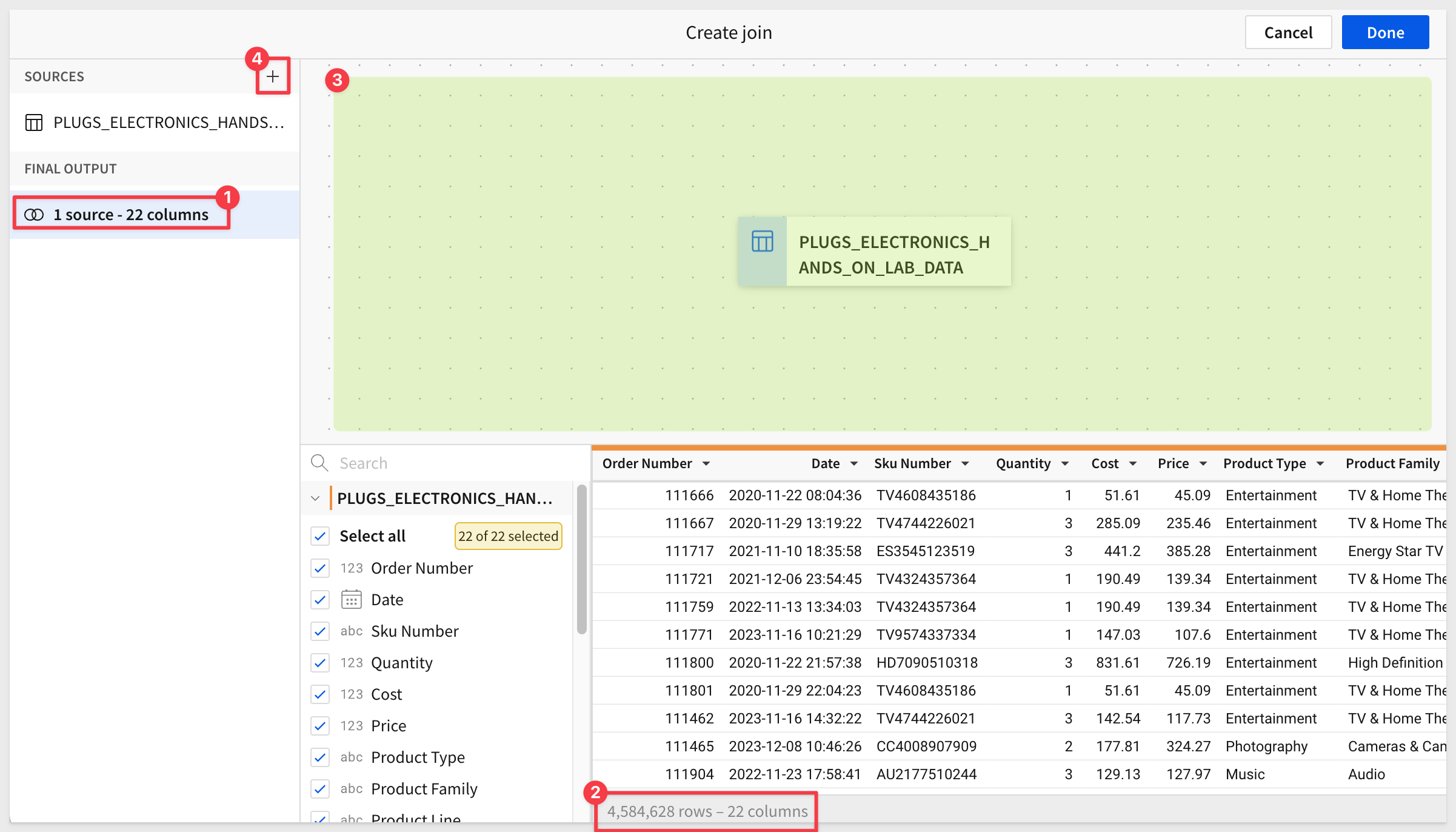
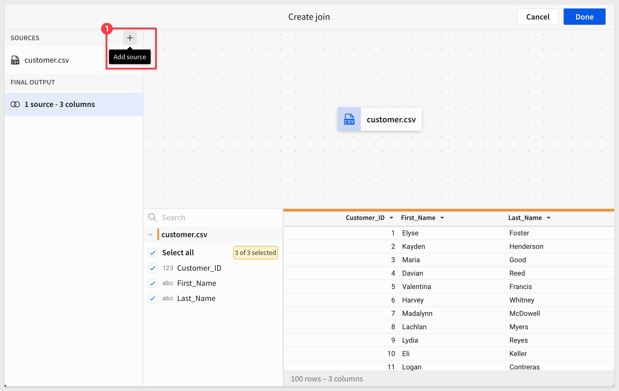
We are now in the Create join interface. At this point, we have 1 source that has about 4.5 million rows of data in 22 columns.
The area in the green is called the lineage and will graphically represent how our data is joined, as we add more tables to the join:
This data currently has retail transaction data, but let assume we want to add additional customer demographic and store data to it. This will allow users to leverage one table to drive a variety of user cases.
We know the data is available in two additional tables, so we need to join them.
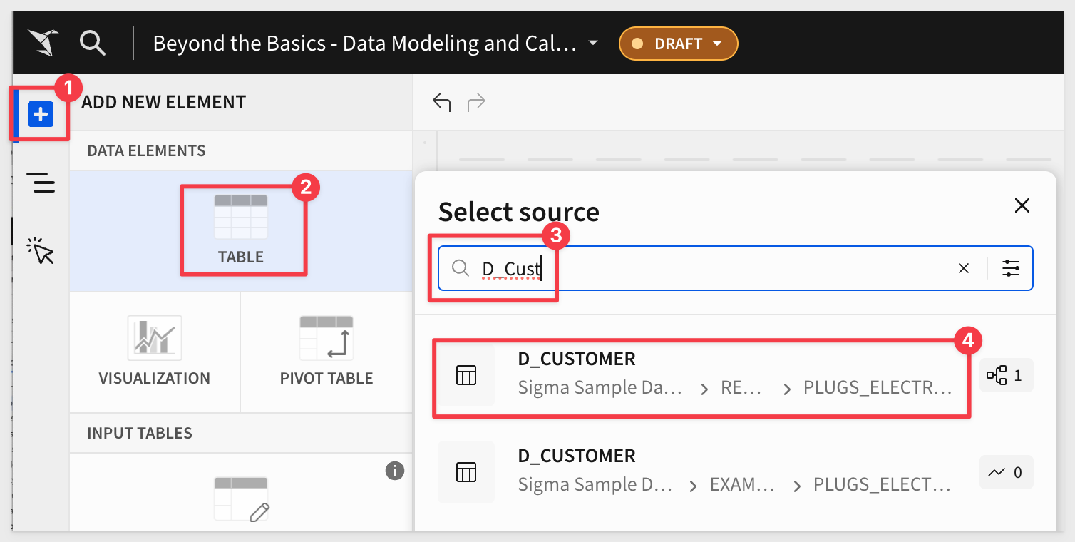
Click the + icon (#4 in the screenshot above).
In the search bar, enter d_customer and select the D_CUSTOMER table:
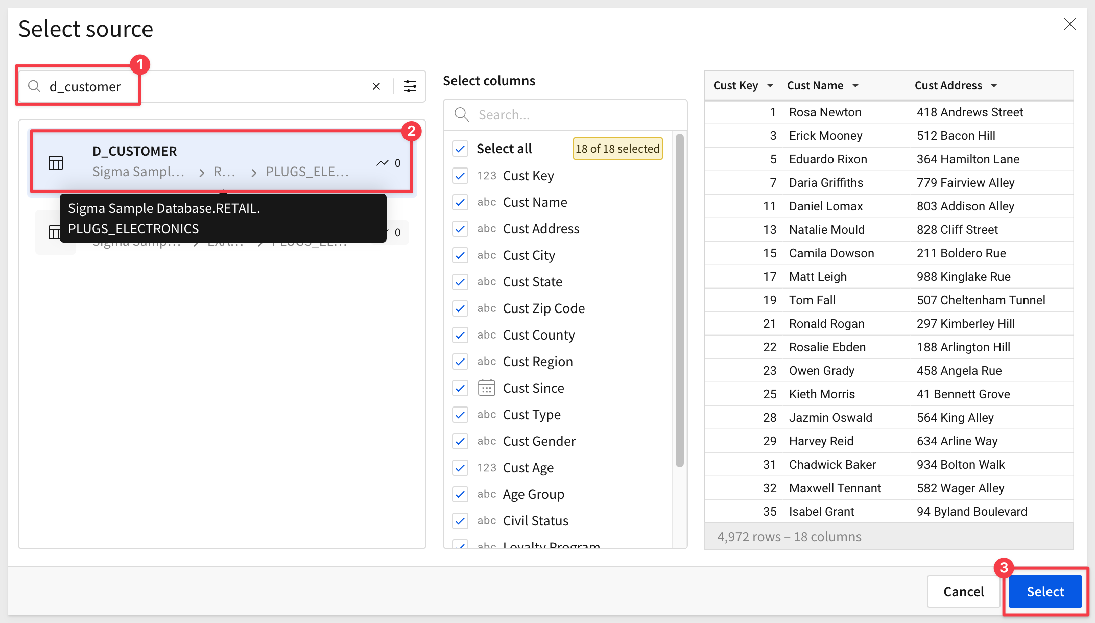
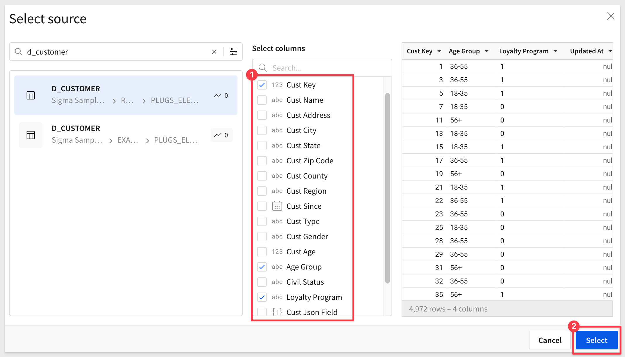
This time, deselect all columns and select only the columns required by the business users. Click Select:
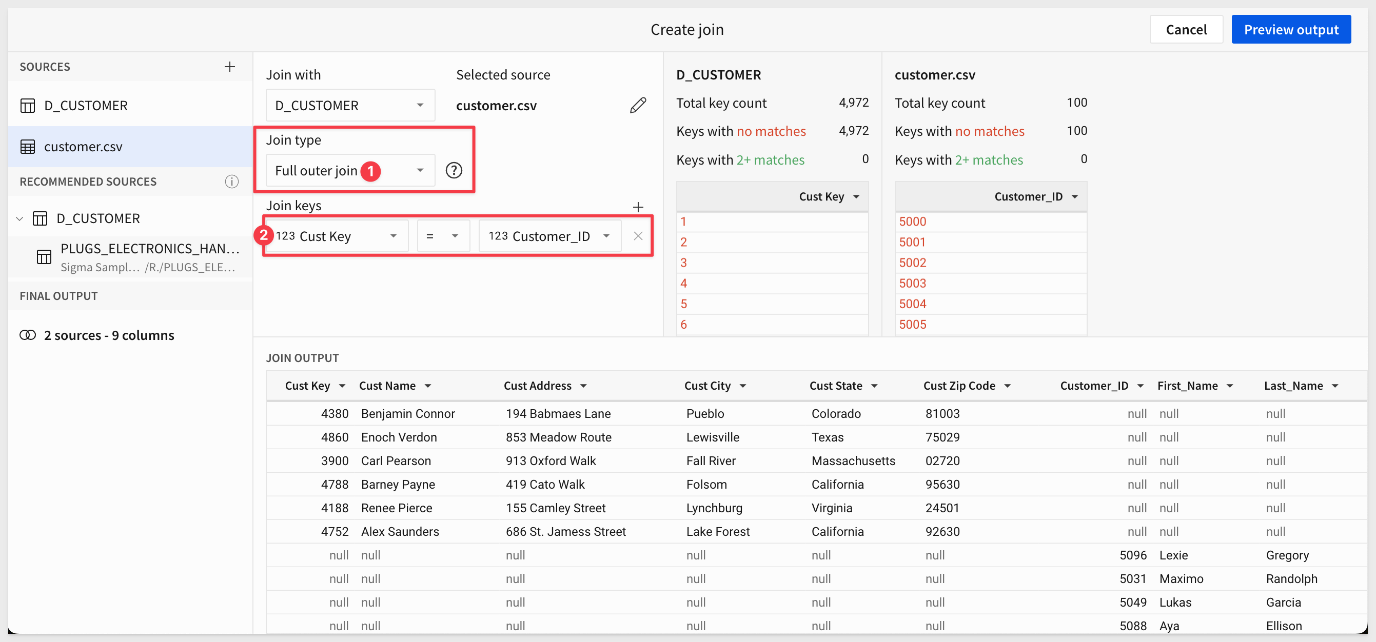
We can now configure the join using a simple interface and avoid having to write custom SQL, although Sigma supports this too.
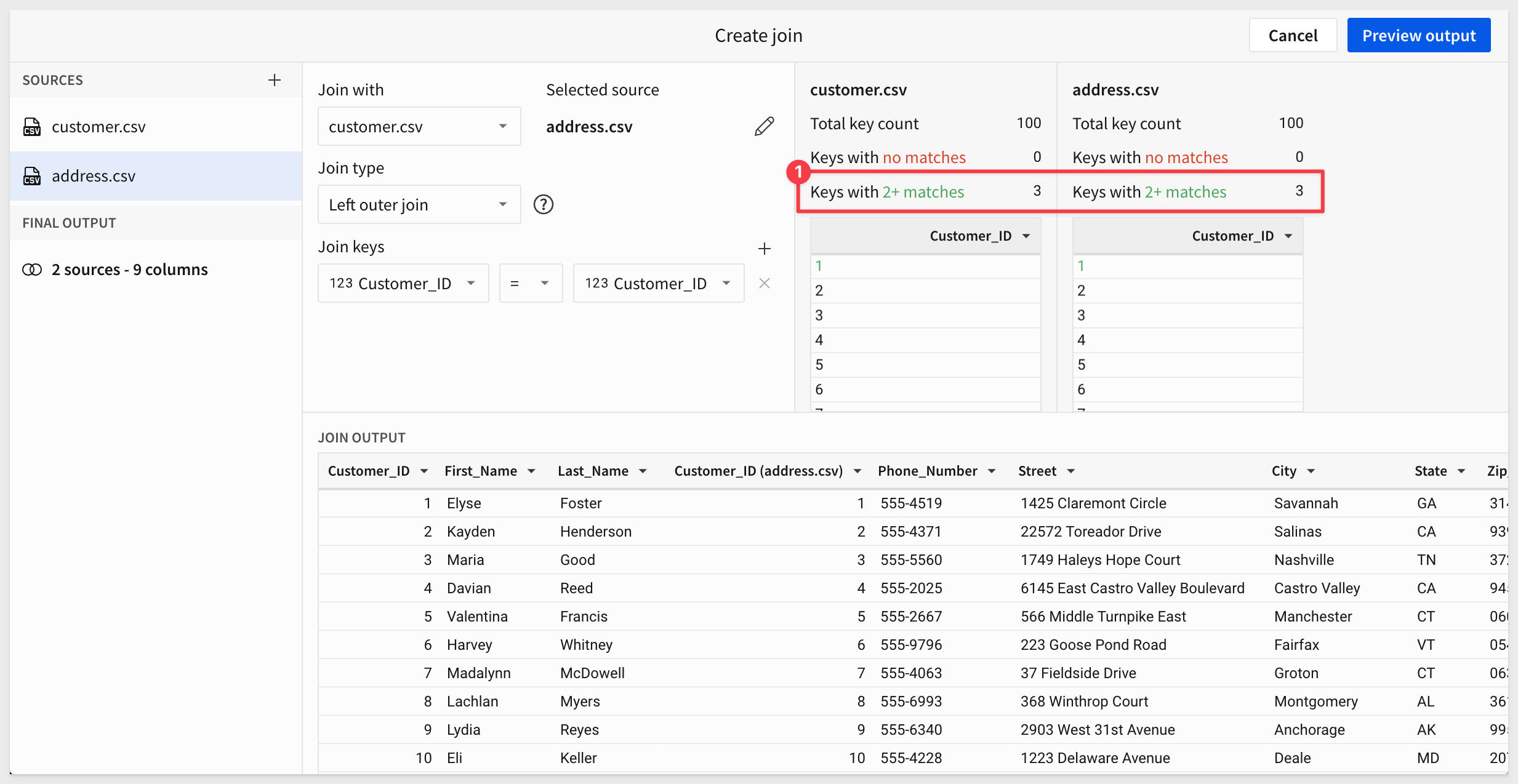
The numbered items in the screenshot below highlight the important elements on this interface.
- 1: The join is 2 source tables with a combined 26 columns
- 2: We are joining
D_CUSTOMERtoPLUGS_ELEC....onCust KeyusingLeft outer join. - 3: For every order in the
PLUGS_ELECTRONICS_HANDS_...sales table, we have a matching customer. There are some customers (105) that have not placed an order.
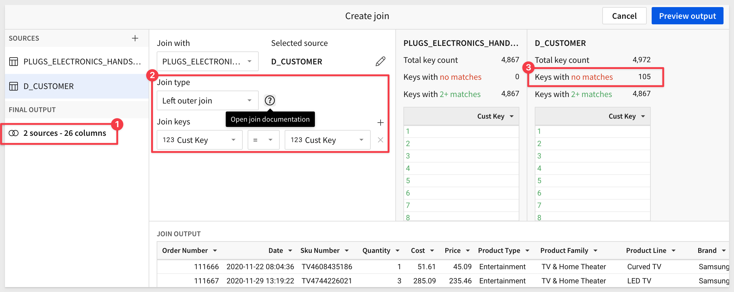
We could now click Preview output, but our requirement was to also provide store detail. Click the + icon to add another table.
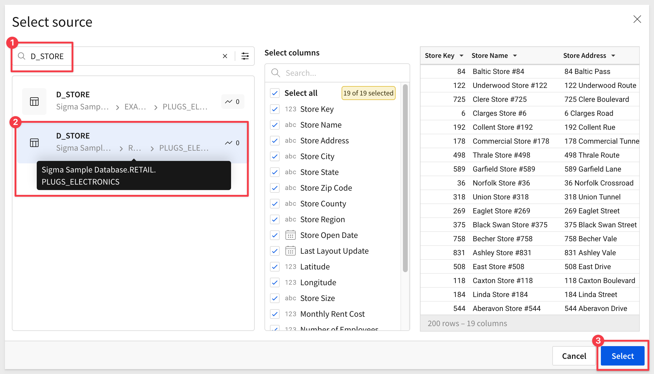
In the search bar, enter d_store and select the D_STORE table:
Make sure to select the D_STORE table from the RETAIL database (there are different sample versions available). We will take all the columns this time; click Select:
We now have 3 sources - 45 columns, are matching on Store_Key, and every sales has a matching store:
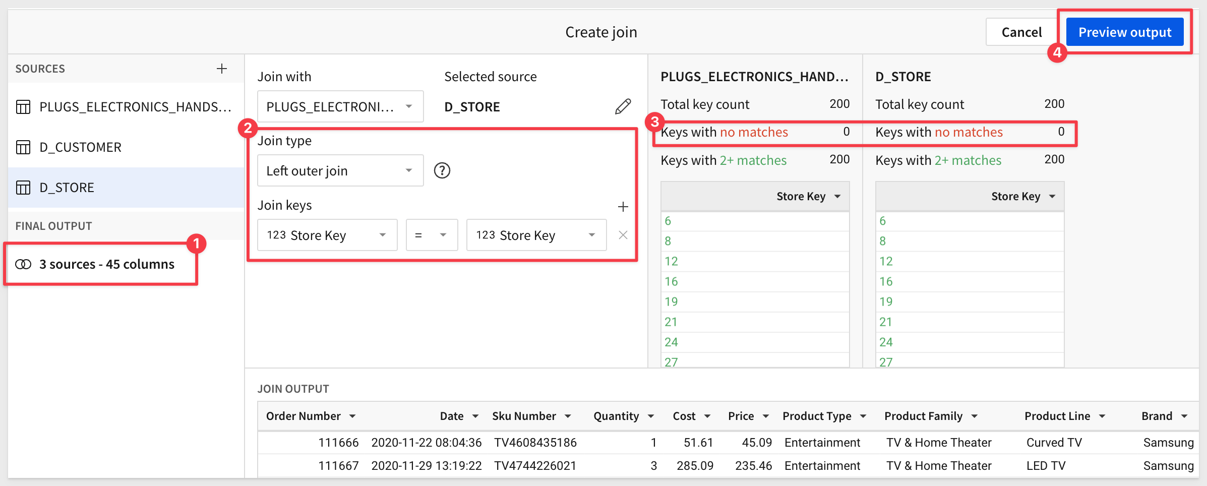
Click Preview output.
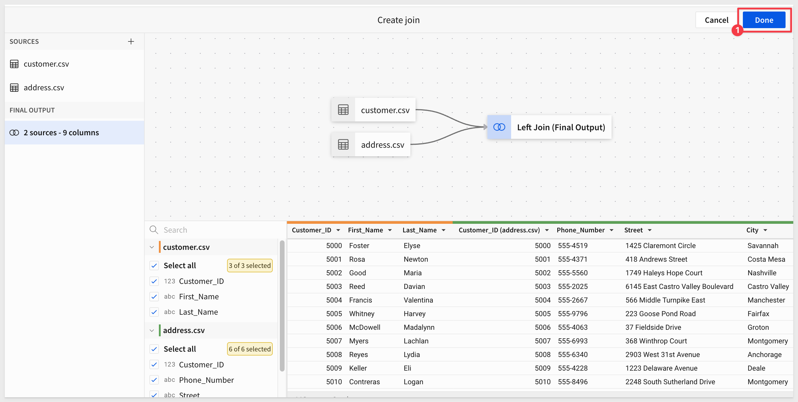
We are shown the updated lineage and have to opportunity to go back and make any changes, if needed.
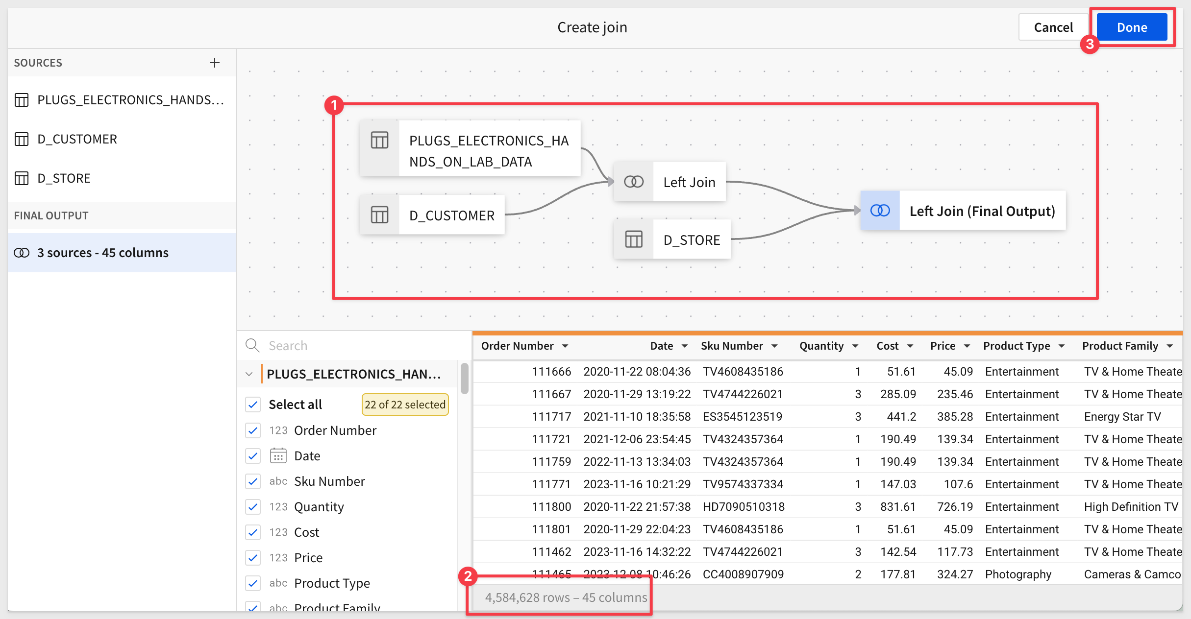
Before we click Done, notice that the row count still has the expected value (around 4.5 million rows) that we had at the start. This makes sense since the base table is retail sales, each sale having a customer and a store.
Click Done.
We are landed in a new Sigma workbook, with our joined tables having a generic name.
Change the name of the new table to something more descriptive. We used Sales Detail | Customer and Store Demographics:
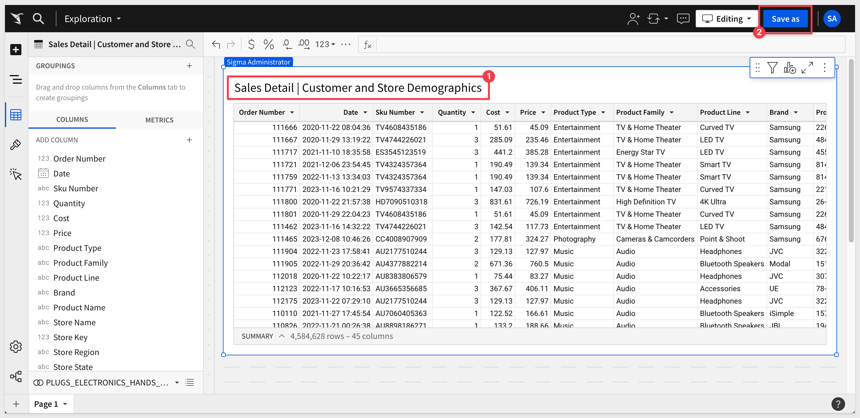
Add a new column, rename it to Sales and set its formula to:
Sum([Quantity] * [Price])
Change the format of the Sales column to Currency.
We need this column in later sections.
Also click Save As and name the workbook Beyond the Basics - Data Modeling and Calculations.
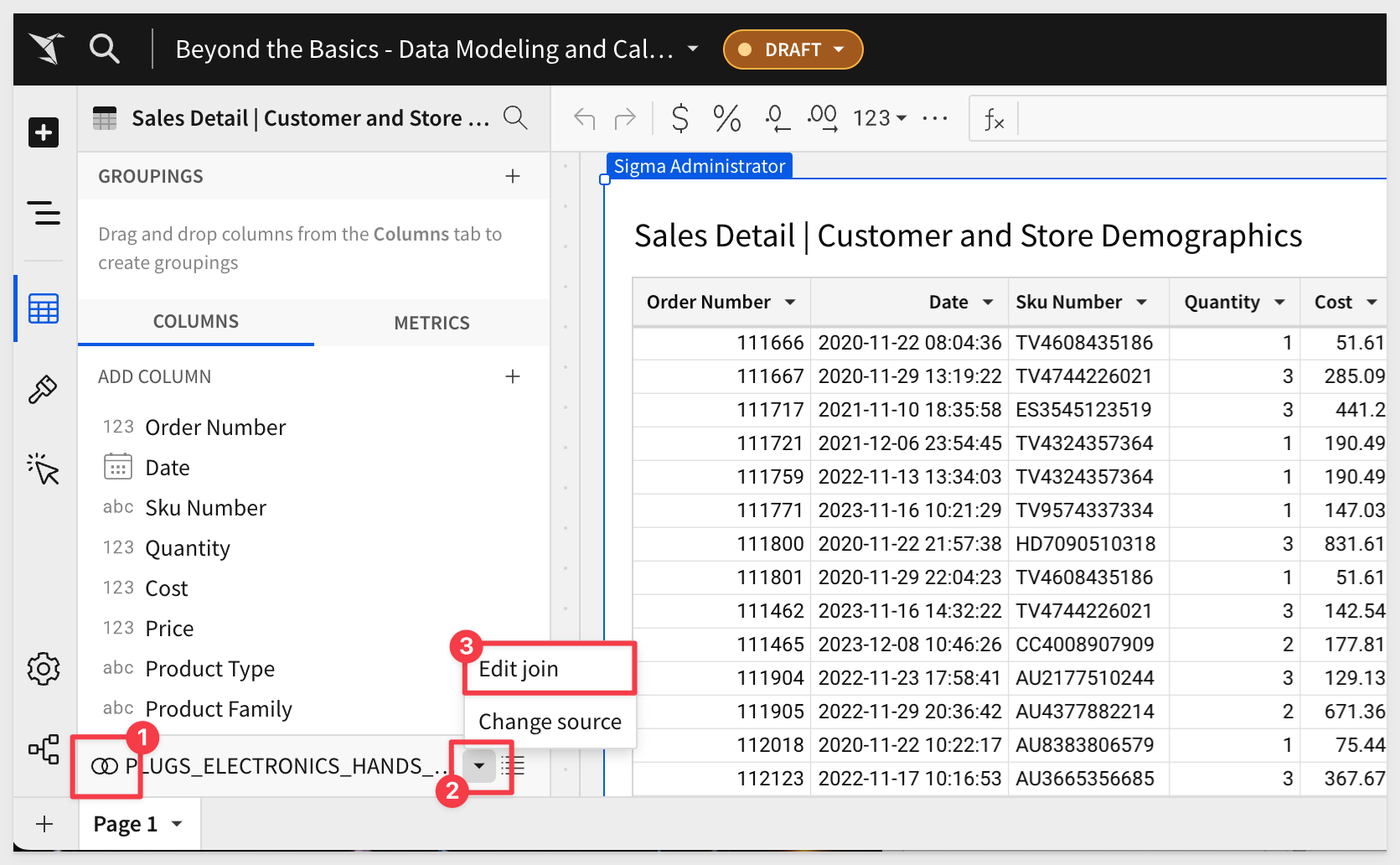
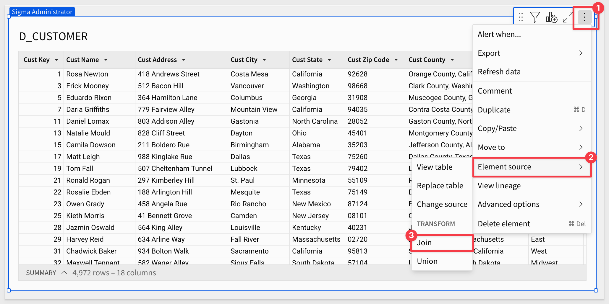
Sigma also makes it really simple to know that this data comes from joined tables (number 1 in the screenshot). Editing the join is equally simple (number 2/3):
Rename Page 1 to Common Join and Publish the workbook.
A common request we get to our support team is how to handle data that is "dirty" or has problems that are exposed as tables are joined together.
While there are many possibilities in this area, we will present a simple example, using two CSV files. When these files are imported into Sigma and joined, there will be duplicate rows. We need to know how to easily identify them, and a method to deal with them.
Before we can do anything, we need to download the sample CSV files. These are really small samples, so the files are equally small in size.
Once the compressed file is downloaded, extract the csv files.
The two files are:
- customer.csv: This is a list of 100 random first and last names with a unique customerID per row.
- address.csv: This is a list of randomly generated US addresses, each with a customerID that corresponds to the customer.csv table.
Marketing promotion
Lets assume that this data is coming from a promotion that marketing is running for new customers only. There is a web site that allows registration, and new customers are informed that they can only register one time for the promotion, although the web site does not actually enforce that restriction.
Sounds pretty straight-forward so far, but lets see what happens when we import these into Sigma and join them together.
Import and Join
We already joined data in the first section, so the steps in Sigma are mostly the same, except this time we will use the csv files as sources instead of Sigma's sample data.
In Sigma, return to the workbook and add a new page. Rename it to Dirty Data.
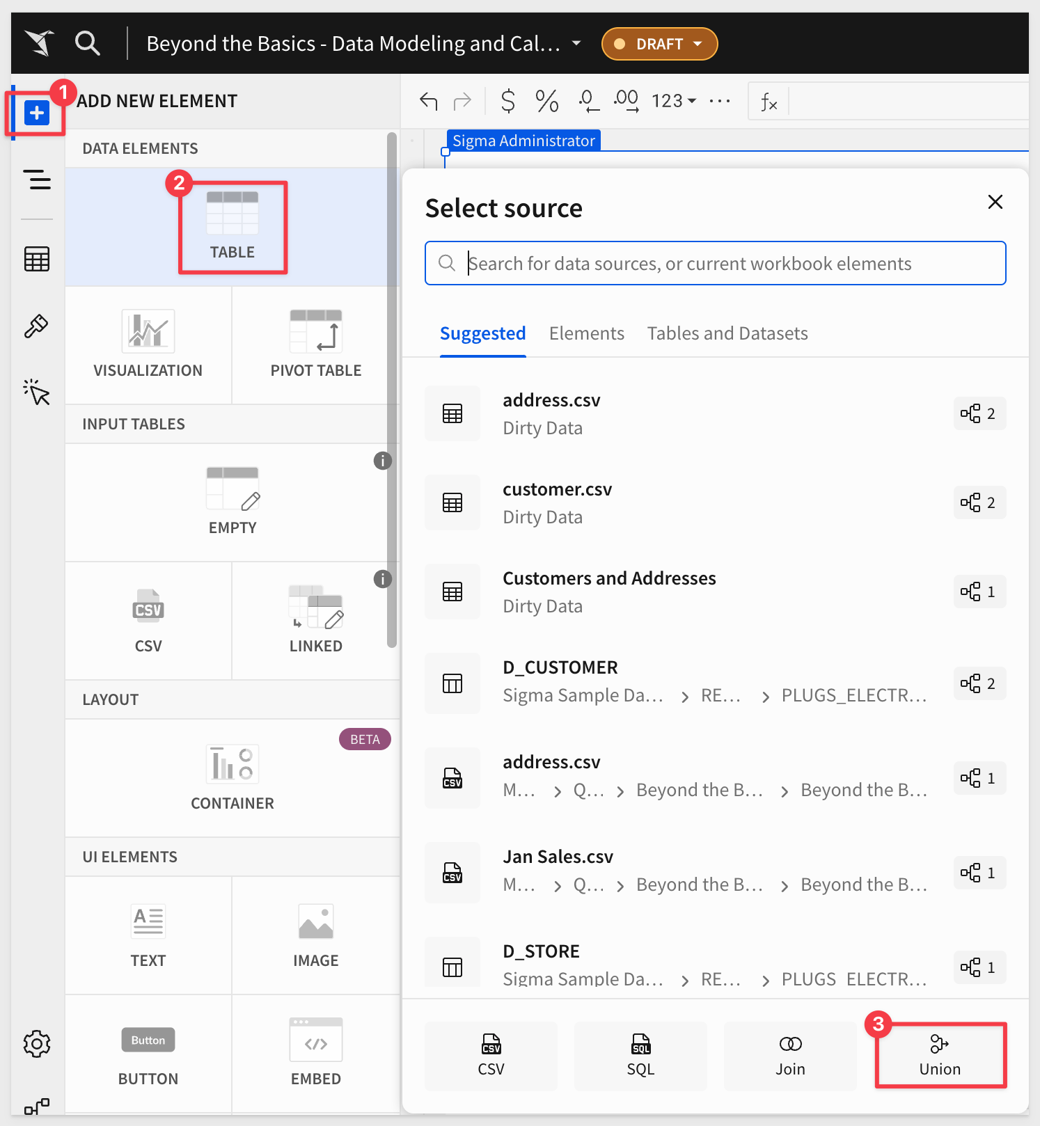
Add a new table to the page, but this time, select the CSV option:
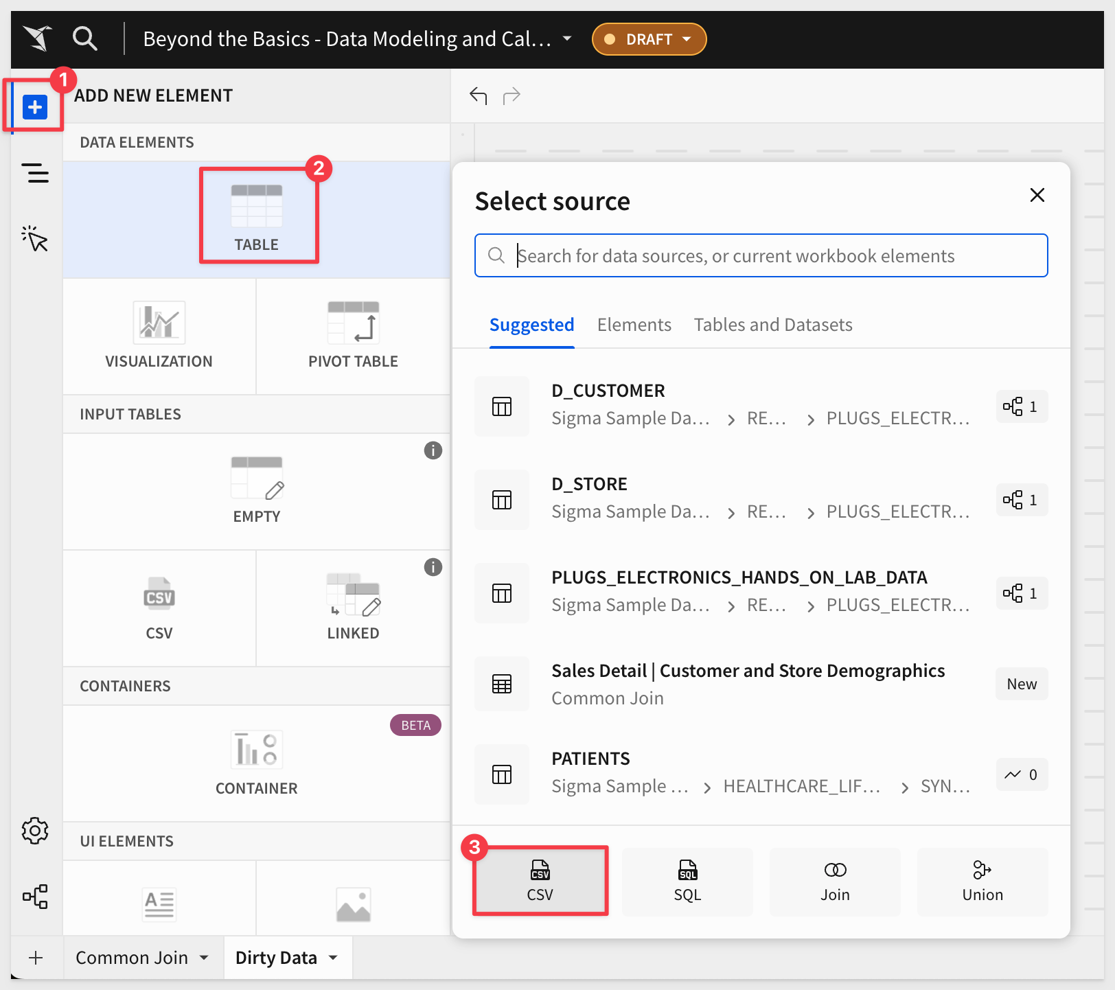
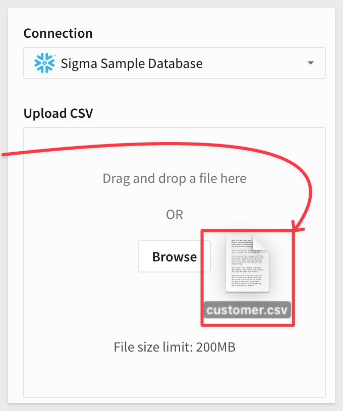
Drag and drop (or browse to find) the customer.csv file from the extracted download:
Sigma will show us the contents of the file. Click Save.
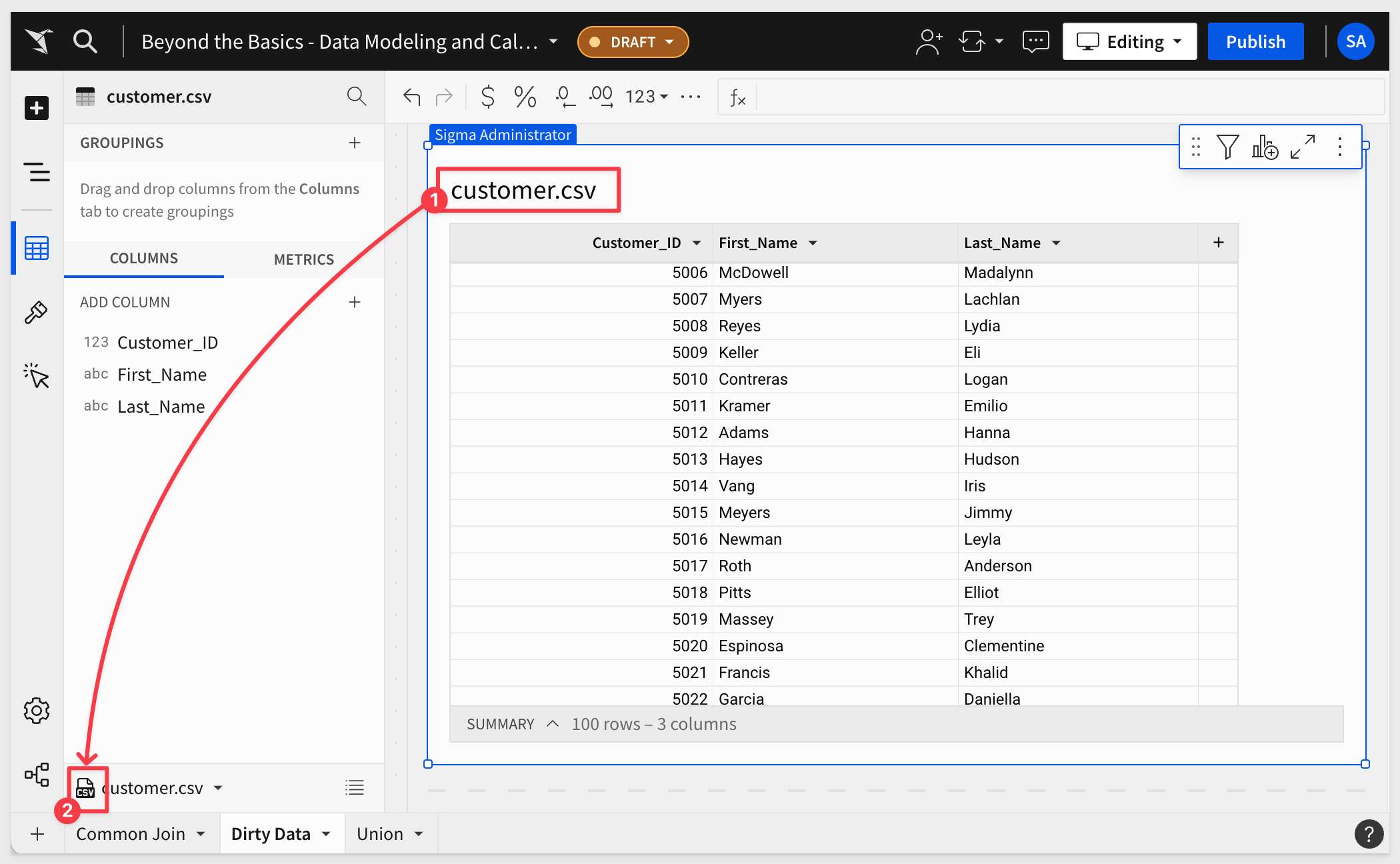
The file is imported and we can see the three columns mentioned earlier. Notice that the icon for the table (#2 in the screenshot) indicating that it's source was a CSV. These icons are good to know.
Repeat the same process, but this time use the address.csv file as the source of data:
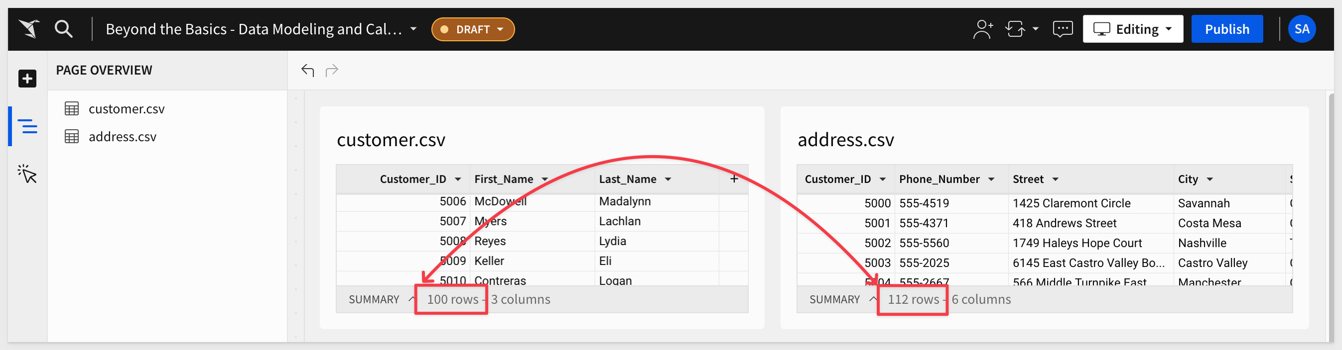
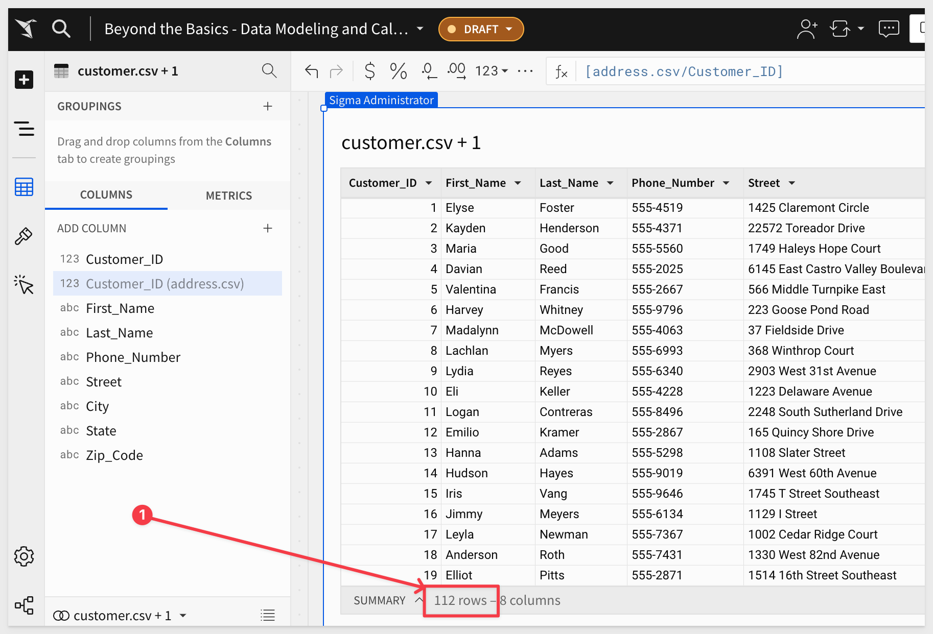
We now have the two files as tables in Sigma. If we take care to observe the row counts for each table, we may notice that there are 100 customers, but 112 addresses. There are cases where that may be fine, however it largely depends on the context in which this data is being used.
While this is a clue that there may be some problems, lets join them and see what happens in Sigma.
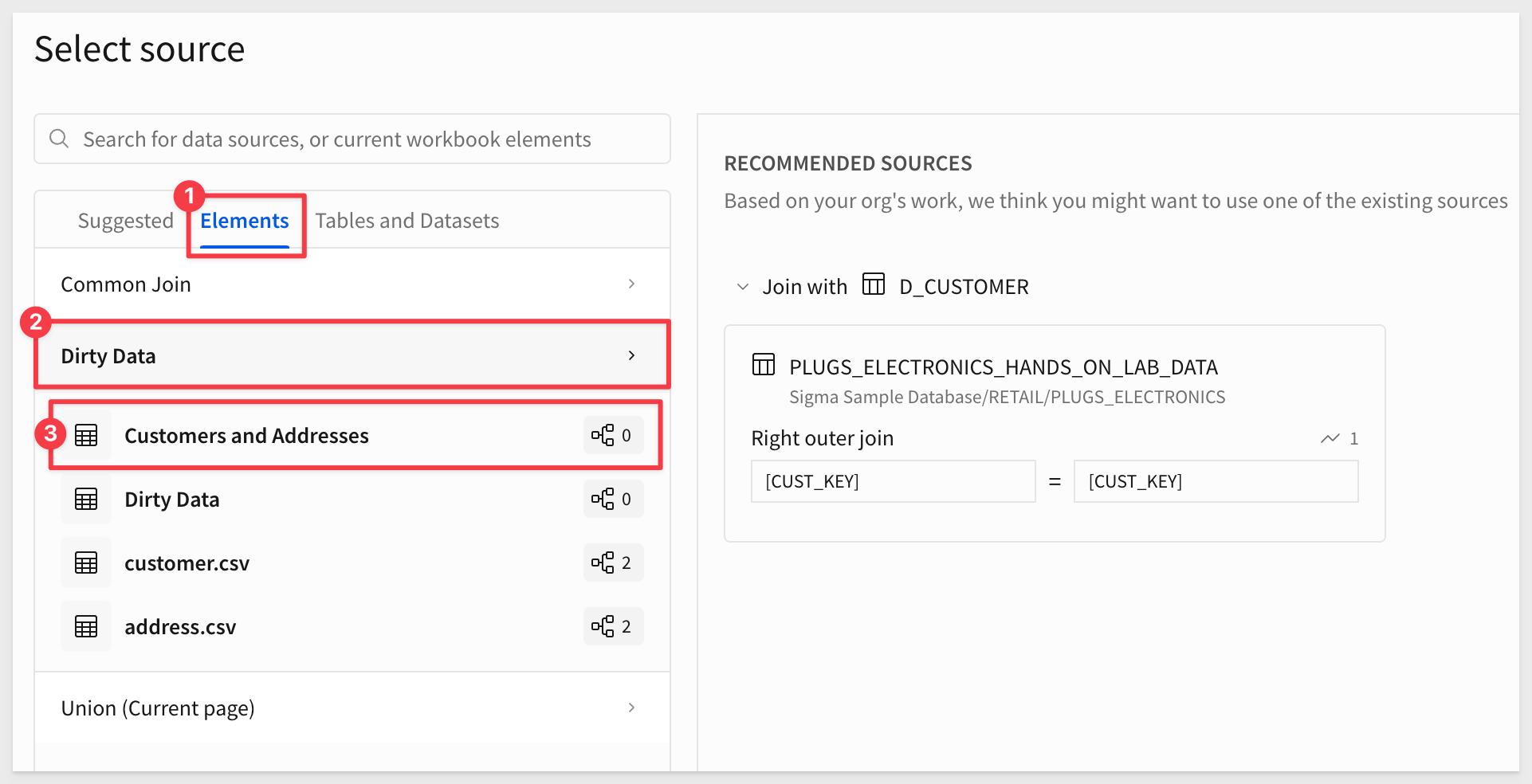
Add another table, but this time select Join as the source:
Our customer.csv table will be on the list under Elements; select that and click Select.
In the Create join interface, click the + to add another source:
Our address.csv table will be on the list; select that and click Select.
We are now in the familiar Create join interface, where we can adjust the join conditions to suit our needs.
We can leave all columns selected, as that is not important for this demonstration.
What is important is that Sigma has identified that there are join keys in both tables that have more than 1 match.
This may not always be a problem as discussed, but is another clue that we need to be ready to verify the results against our expectations.
Click Preview output and then Done on the next (lineage) screen:
Identify, Organize and Action
Lets dig deeper into the data and see what we find.
Rename the new table to Customers and Addresses for clarity.
Sorting
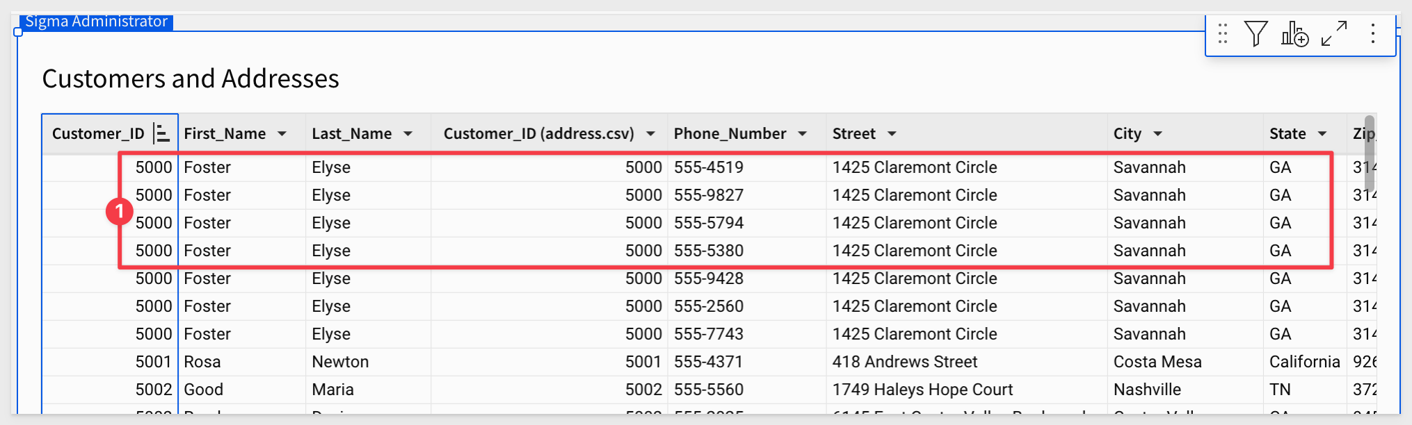
Sort the table, ascending on CustomerId.
We can now see that CustomerID 5000 has multiple entries, and upon closer inspection has registered the same address with different phone numbers:
Grouping
Grouping the table on Customer_ID we can now scroll down to see which other customers have multiple entries in the table.
For example, CustomerID 5049 and 5054 both have more than one entry:
One path forward
How can we address the extra registrations and report the ‘dirty data' back to the data team, so they can clean it up at the source as well?
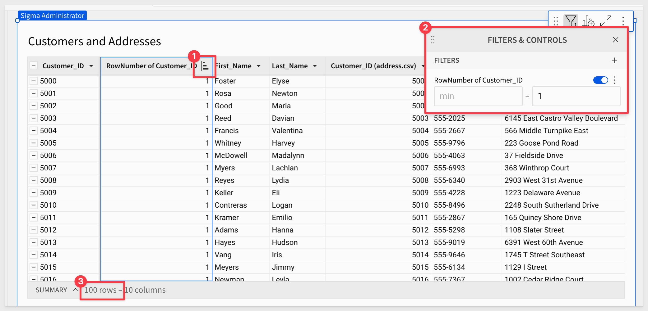
There is a simple way to handle the extra registrations that resulted from the join, using the RowNumber() function.
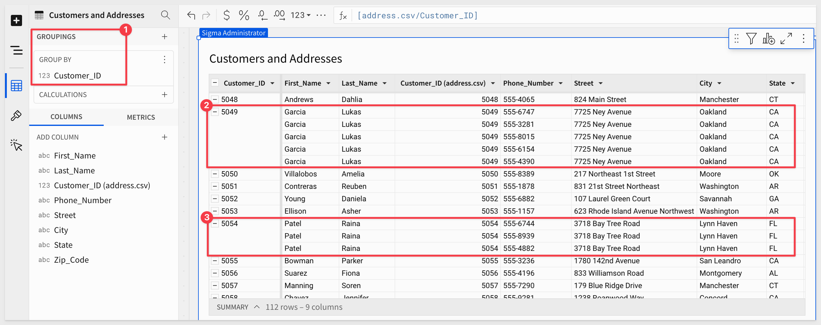
Add a new column outside of the grouping set its formula to:
RowNumber([Customer_ID])
Sort the table by the new column:
Now we can see how many times each Customer_ID appears in the table.
Additionally, we can filter on the new Row_Number column, and set the maximum value to 1, to filter out the extra rows.
Notice that we now have the expected 100 rows of data too:
While this may solve our immediate needs, it doesn't resolve the dirty data issue and it would be ideal if we could help with that too.
Duplicate the Customer and Addresses table and rename the new table to Dirty Data:
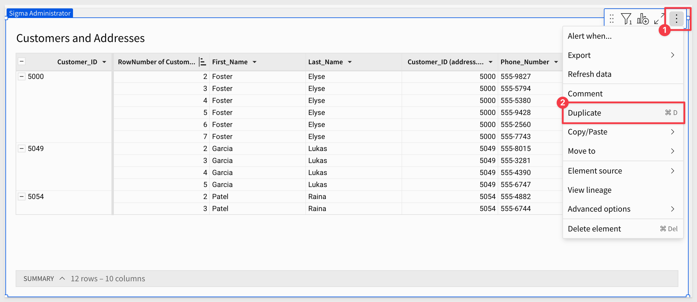
Set the filter on the Dirty Data table to show only the "bad" rows:
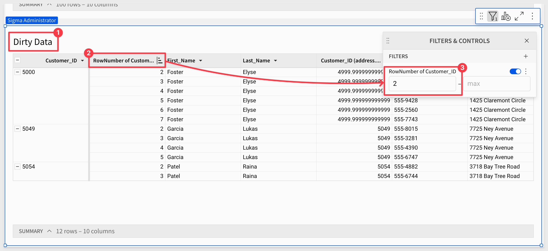
These are the 12 registrations we want to alert the data team about.
Publish the workbook.
Conditional alerts
Lets assume this is a workflow that will run for some time, with new records being added as new customers register for the promotion.
We want to both alert the data team and attach the new records that have more than one entry for the same Customer_ID (for example).
Now we can simply click the dropdown arrow next to the title, select a Schedule exports and share this with the data team, if the table has any data:
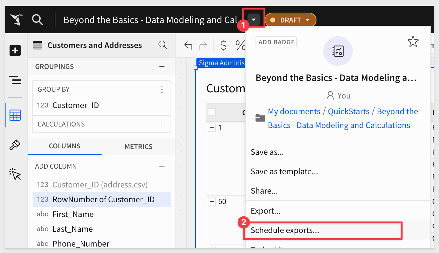
After clicking Add schedule, we want to enable Condition and the rest is very straight-forward:
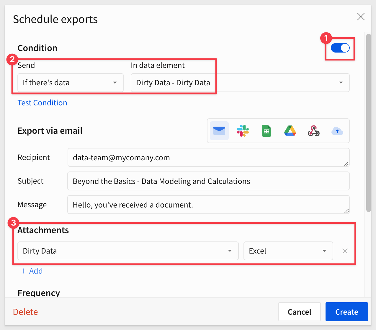
Based on our schedule, anytime there are new extra rows in the Dirty Data table, the data team will get an email with the list attached in Excel. Of course, there are other methods supported too, so that the process of remediation can be automated to suit your organization's needs.
To learn more about scheduling exports, see here.
Another very common use case is finding the data that is common between Table A and Table B, what appeared in Table A that did not appear in Table B, and vice versa.
For example, maybe we want to find customers (common to both tables), new customers (unique to Table B), and churned customers (unique to Table A).
Using unions in Sigma is very simple, and the workflow is basically the same as we have already done.
In our use case, we have already found and handled customers who registered multiple times. However, our promotion is for new customers only, so we need a way to check against our existing customer table too.
Create a new page in our Beyond the Basics - Data Modeling and Calculations workbook, and rename it to Full Outer Join.
Add the D_CUSTOMER table to the page:
Now that we have D_Customer, we can add a join directly from it:
In Elements, select the Customers and Addresses table from the Dirty Data page:
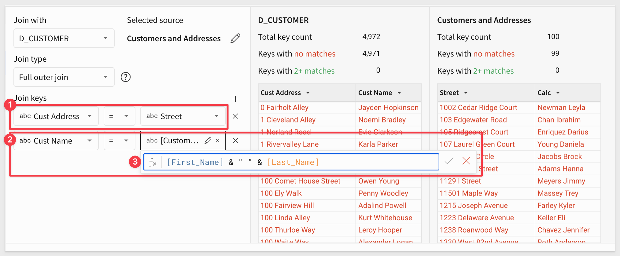
Set the Join type to Full outer join:
Our Customers and Addresses table will not have Customer_ID values that match to our D_Customers table, as they are coming from our website promotion, which was unaware of our internal customers data.
In our use case, we want to ensure that the person registering is not an existing customer, so perhaps we can check their name and address against our existing customer data to see if there is a match (for example). While this may not be a perfect method, it will get us close enough for this demonstration.
Set the Join keys to:
Cust Address = `Street
To avoid people with the same names, we need to add a second Join key and use a custom formula that concatenates the first and last names of the customer in the Customers and Addresses table, since they are separate columns:
[Cust Name] = [First_Name] & " " & [Last_Name]
For more information about operators in Sigma, see here.
Click Preview and Done.
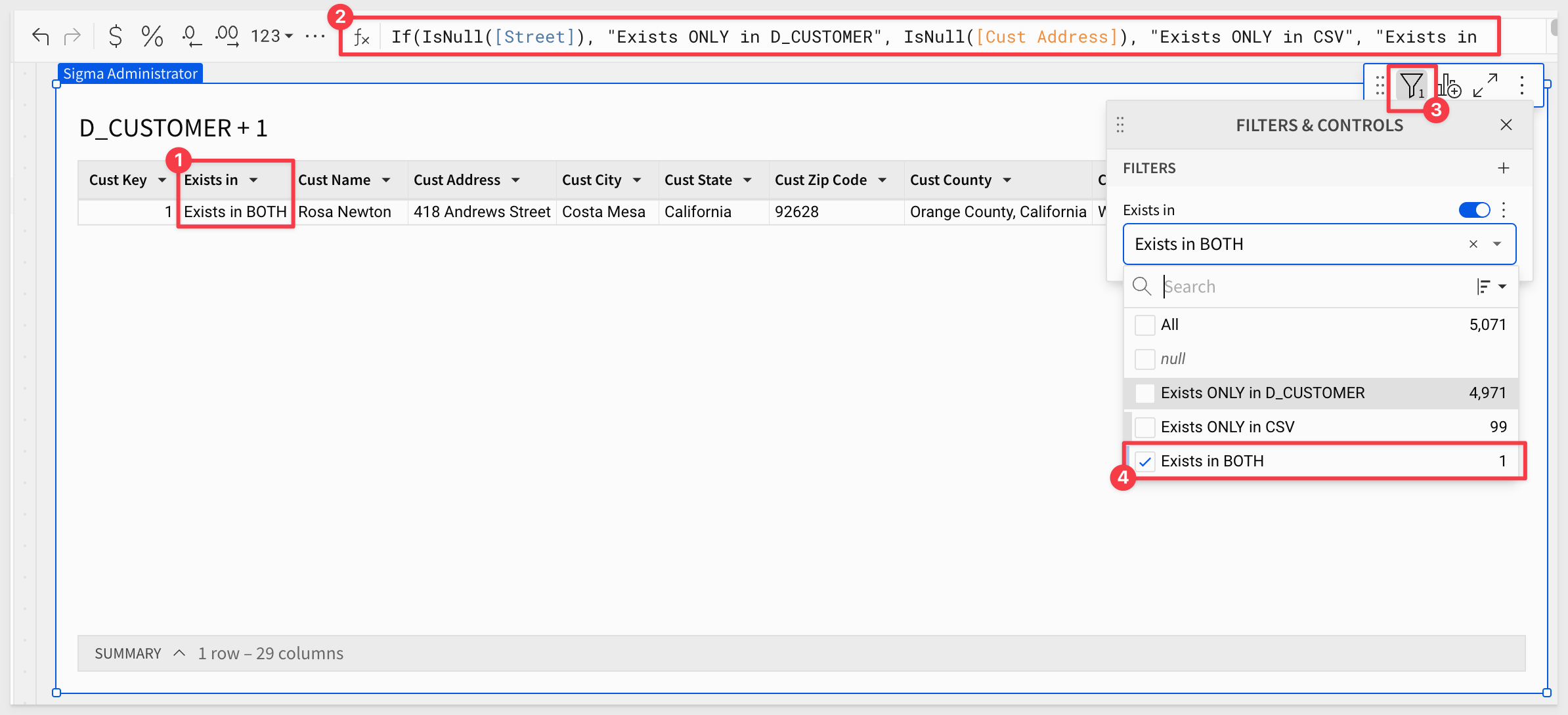
Add a New column, rename it to Exists In and set its formula to:
If(IsNull([Street]), "Exists ONLY in D_CUSTOMER", IsNull([Cust Address]), "Exists ONLY in CSV", "Exists in BOTH")
This formula is used to determine where a particular record exists by checking if certain fields are empty (null).
It returns the custom text if a record exists only in the D_CUSTOMER table, only in the CSV file, or in both.
Set a filter on the new Exists in column and check the box for Exists in both:
We can now see that there is one row of data that is common to both, which means that this user both registered for the promotion and is an existing customer.
Not only was this pretty simple, it underscores some of the power of Sigma, should it be required.
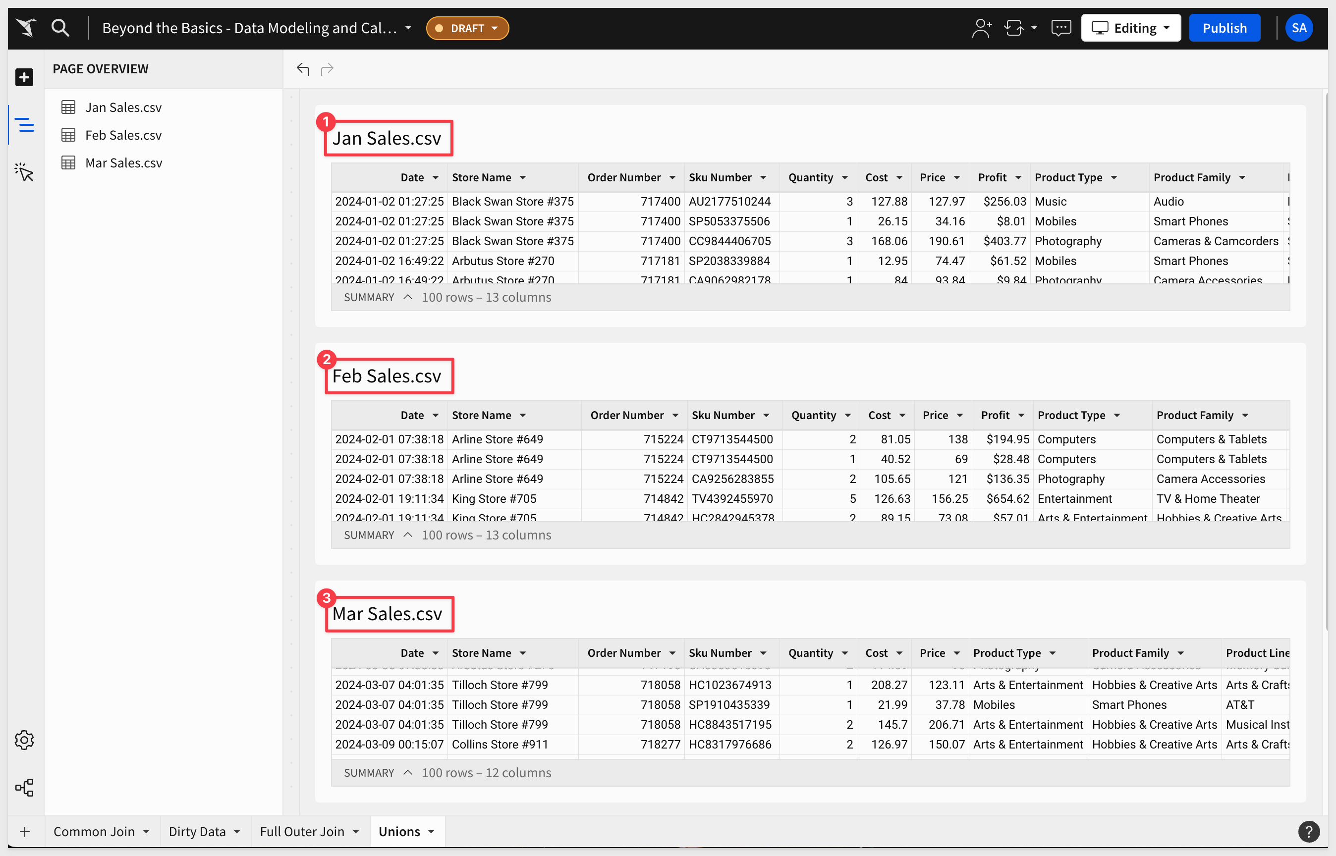
For this demonstration, lets assume that each month we receive sales data for the previous month in .CSV format. We need to report against the quarter, so we need to first join this data together.
We have previously added table elements based on .CSV file uploads, so we can do this ourselves now.
Create a new page in our Beyond the Basics - Data Modeling and Calculations workbook, and rename it to Union.
In our sample data that we downloaded earlier, upload the three .CSV files as new tables. When done, our new page should look like this:
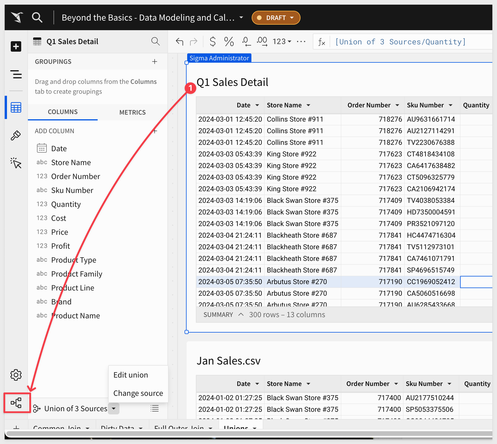
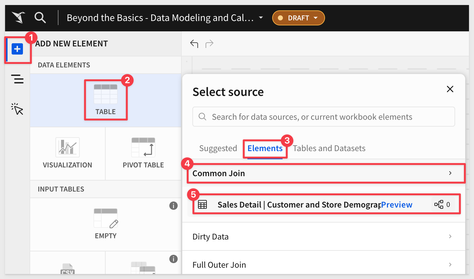
Now that we have the data in Sigma, we can add a new Table and select the Union option:
For the source of data, we will use the tables we just imported:
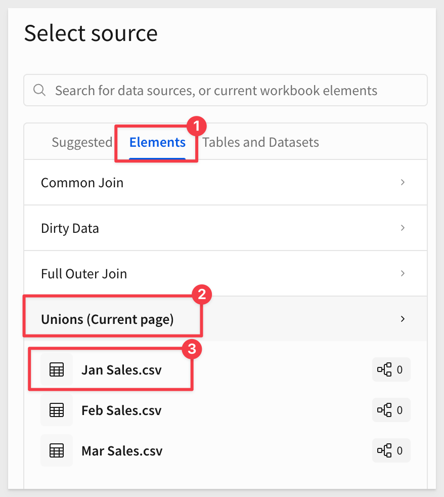
Because we selected Union, Sigma now gives us the option to add more sources:
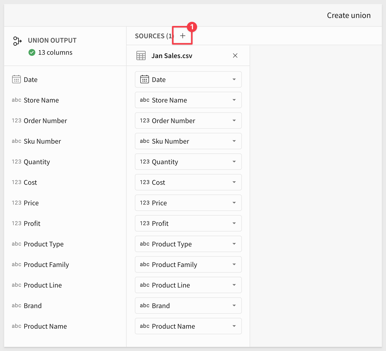
This page also allows us to change the column mapping should it be required.
Click the + to add the next source table, this time selecting the Feb Sales.csv table.
Repeat the process one more time to add the Mar Sales.csv table. The result will look like this:
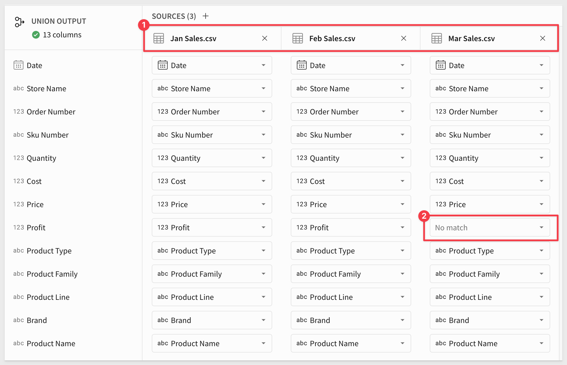
Notice that there is no match in the Mar Sales.csv data for Profit?
While this is a problem, we can still complete the union. Sigma will add null values to the cells with no match.
Click Done.
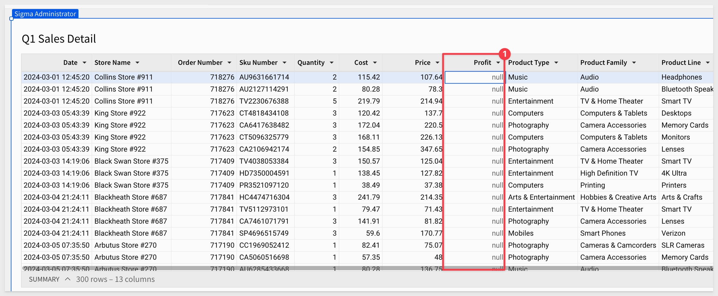
Instead of reporting the issue, we can simply change the Profit column's formula to calculate the correct profit:
([Price] * [Quantity]) - [Cost]
Now we have the data for the quarter, ready for analysis.
Rename the new table Q1 Sales Detail.
Click Publish.
Lineage
As workbooks become more complex, it can be really useful to see graphically see how the data is sourced.
Sigma provides this Lineage automatically and it is accessed by clicking the icon in the lower corner of the workbook:
Because we had the Q1 Sales Detail table selected, the lineage is focused on that:
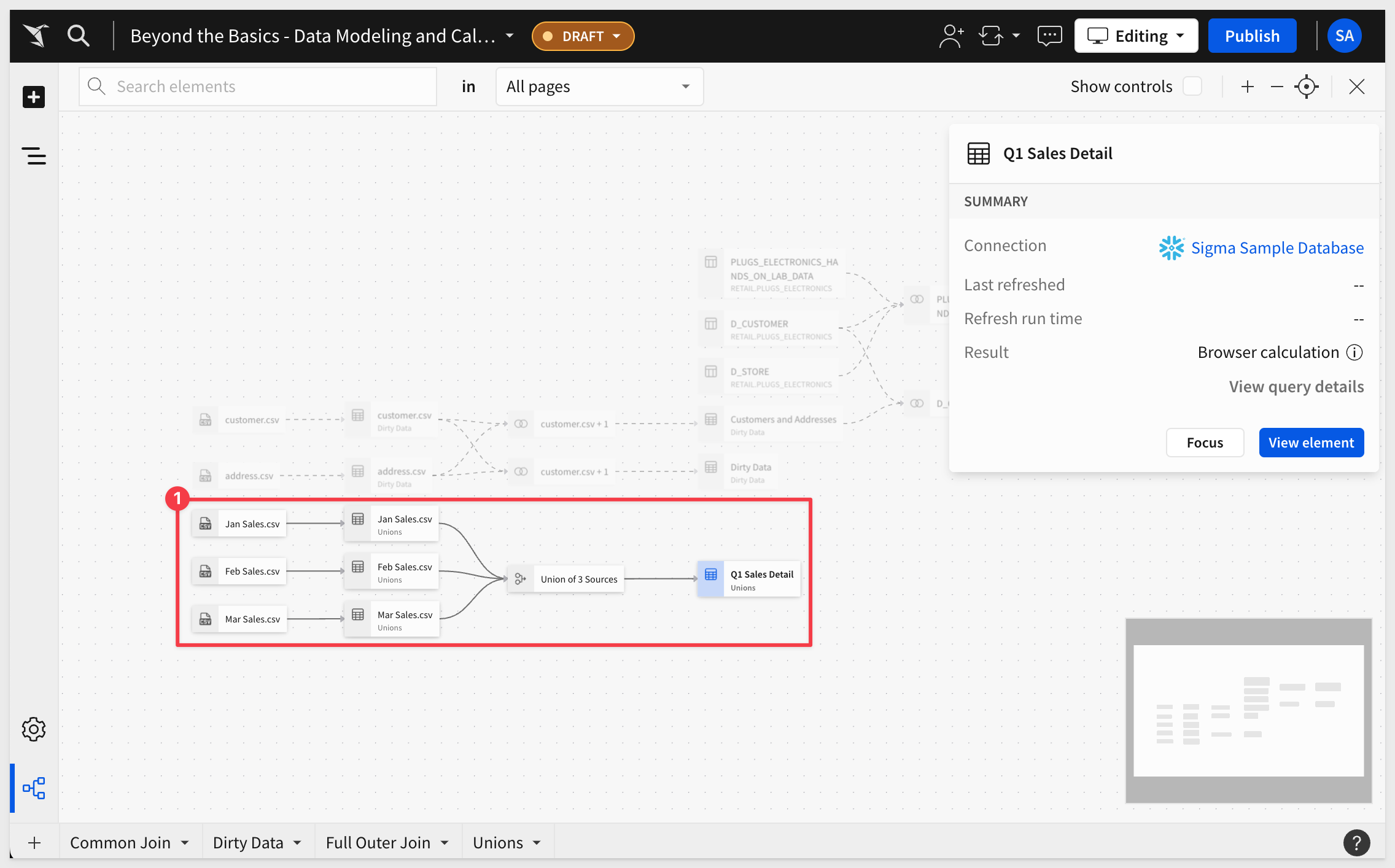
For more information on using lineage, see View workbook data lineage.
If you have ever had to do "date math" in SQL or other tools, you have probably found it frustrating. It can be really challenging at times, as it requires both a good understanding of the data and the proper use of tools to ensure the correct result.
Sigma has added functionality to directly address this, giving users a simple workflow to make it easy, while retaining the ability to manually adjust calculations too.
Create a new page in our Beyond the Basics - Data Modeling and Calculations workbook, and rename it to Period over Period.
Add a new Table element to the page, reusing the Common Join > Sales Detail | Customer and Store Demographics table on the Common Join page:
Rename the new table Period over Period.
Now click on the OrderID column's menu and select Add column via > Period over period comparison"
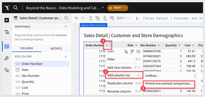
This provides us a simple way to Add Comparison to our table.
We can easily sum Sales and also select to compare the Date columns value to the Same quarter last year:
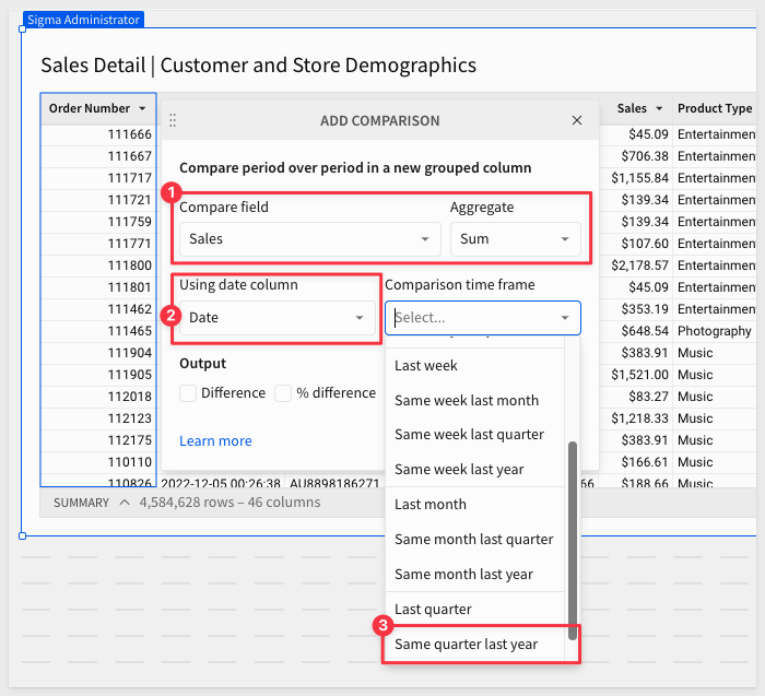
Also check the Output boxes on for Difference, % difference and Value. This will create columns for each of these options.
Click Done.
What happened?
Sigma grouped the table by Quarter of Date (number 1 in the screenshot below) and added the results of three new calculated columns (number 2).
Click the + icon (number 4) to collapse the table's detail data:
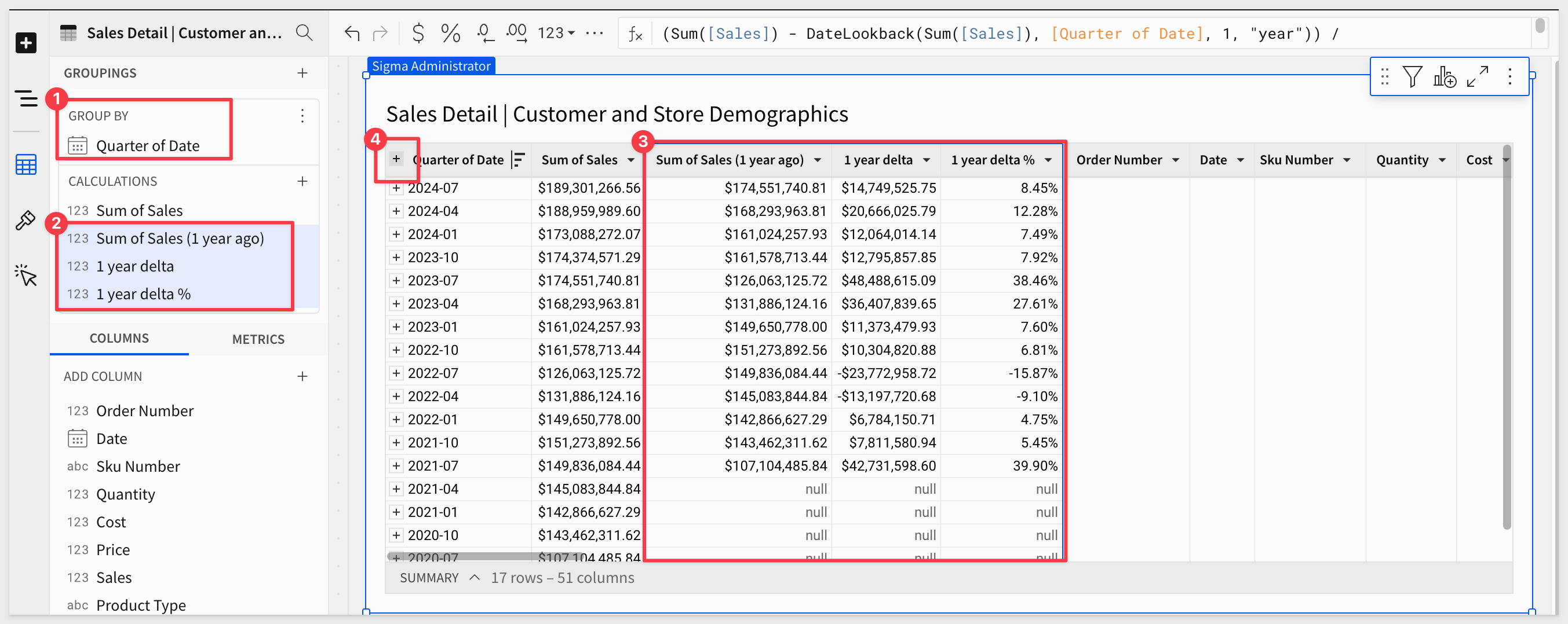
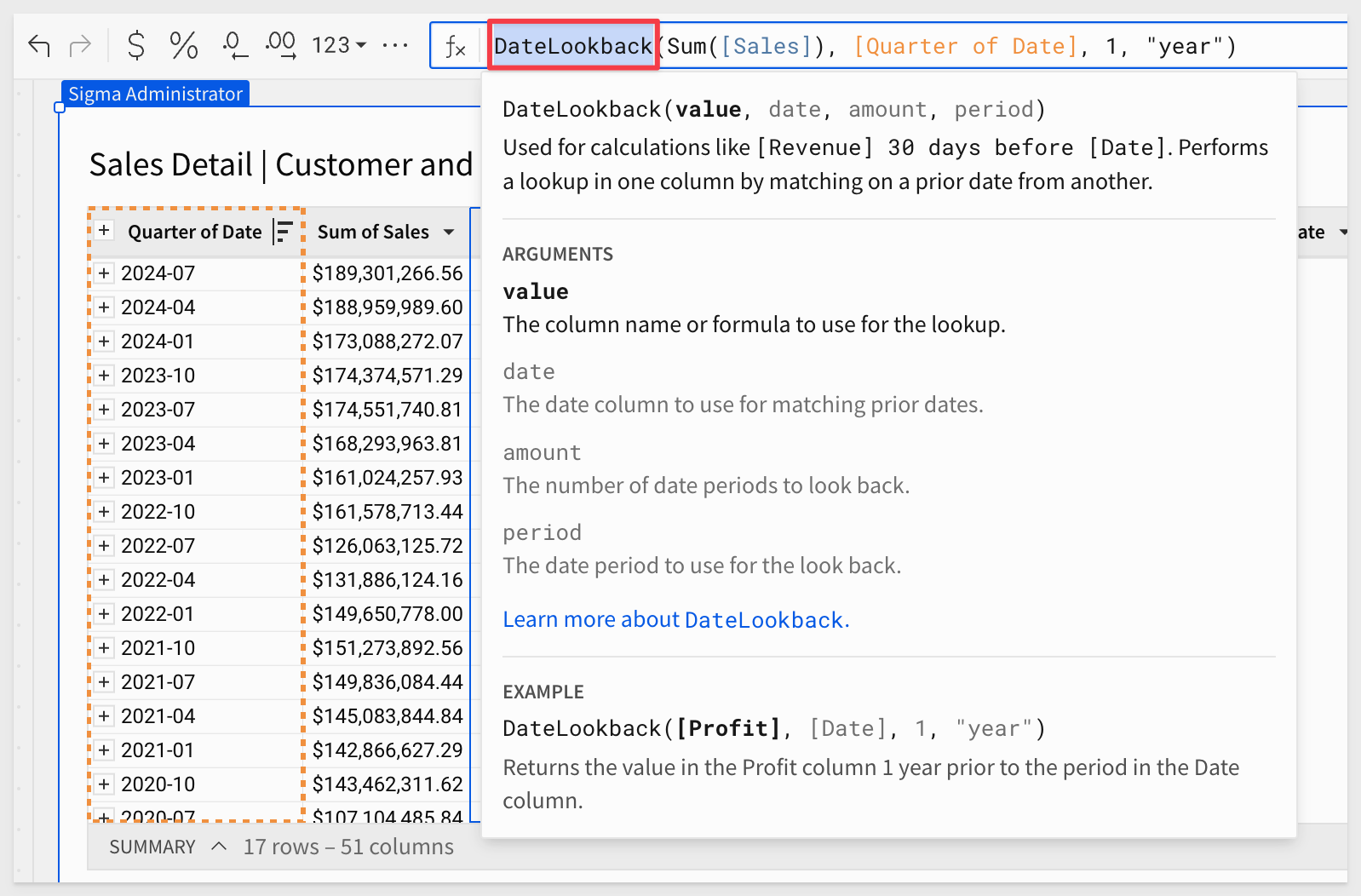
Click on the column Sum of Sales (1 year ago) to see its formula, which is:
DateLookback(Sum([Sales]), [Quarter of Date], 1, "year")
The Sigma function DateLookback is what is working behind the scene to make this possible.
If you need more information on functions in Sigma, we have included a link for your convenience:
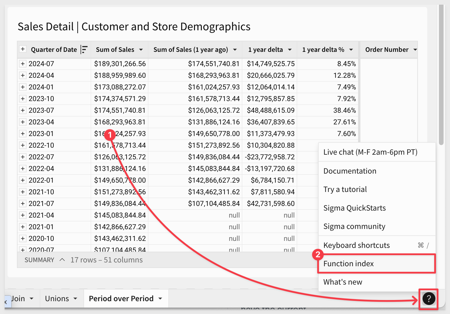
There is also a QuickStart on Common Date Functions and Use Cases.
Publish the workbook.
The cumulative sum function in Sigma helps solve problems related to tracking the running total of a set of values over time or across a sequence of data points.
This is particularly useful in scenarios where you want to observe trends, changes, or cumulative impacts over a period.
By using the cumulative sum function, Sigma allows users to convert individual data points into an aggregated running total, which provides a clearer view of trends and patterns over time, making data analysis more insightful.
For example, you may need to analyze cumulative sales figures to understand how sales build up over days, weeks, or months, allowing for better forecasting and performance tracking.
Lets dig into that example, using our sample data.
Create a new page in our Beyond the Basics - Data Modeling and Calculations workbook, and rename it to Cumulative Sum.
Add a new Table element to the page, reusing the Sales Detail | Customer and Store Demographics table on the Common Join page.
Rename the new table Cumulative Sum.
Add a new column and set it's formula to:
DatePart("year", [Date])
This will give us just the year from the Date column.
Repeat this for another new column and set the formula to get the month this time:
DatePart("month", [Date])
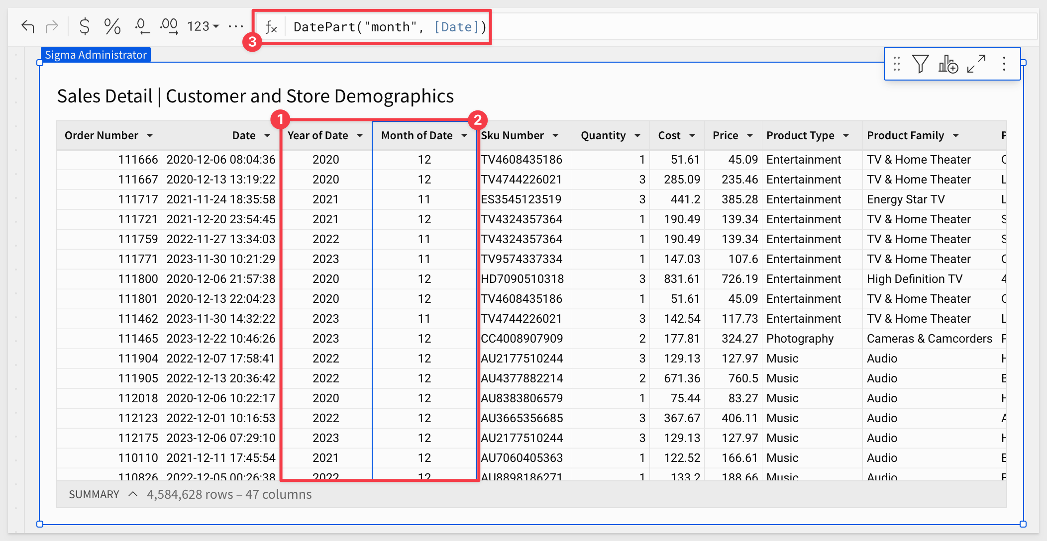
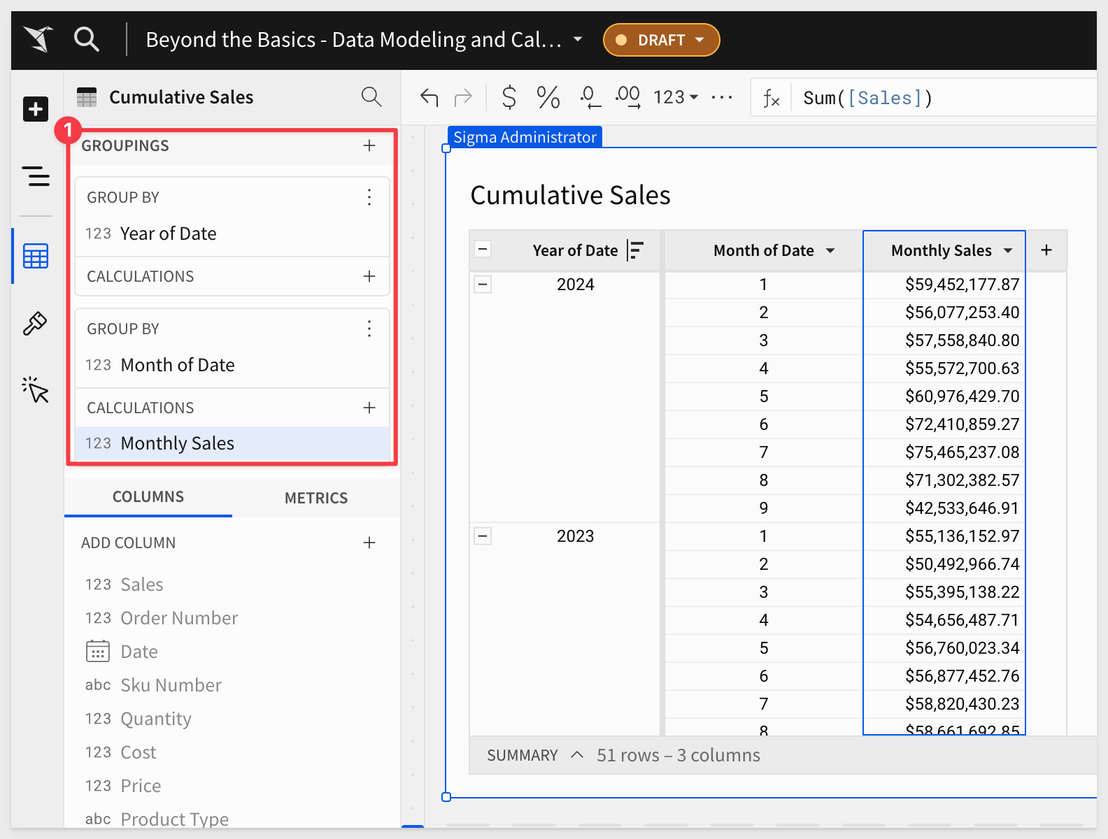
Group the table by Year of Date:
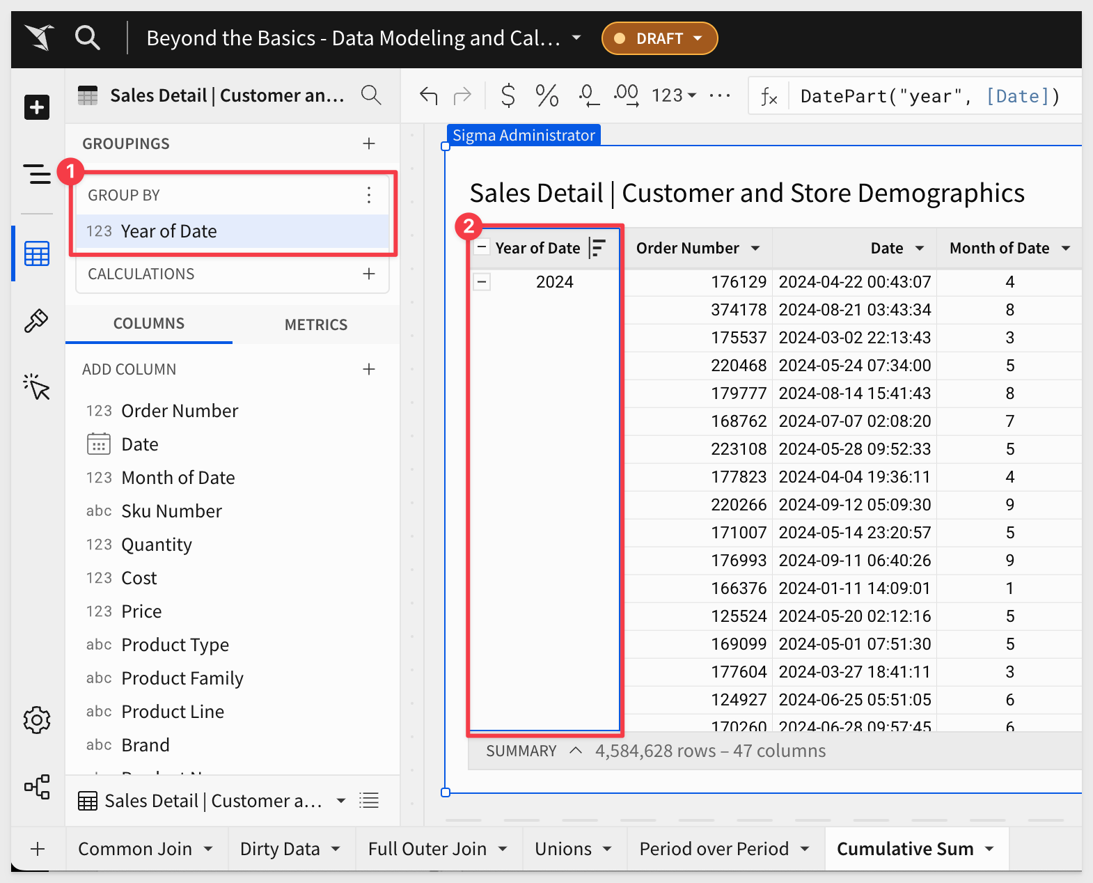
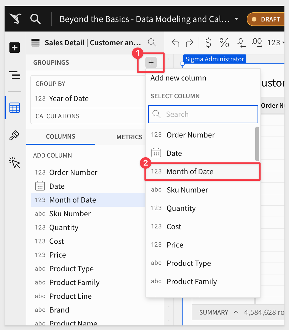
Add another Grouping, this time using Month of Date:
Add the Sales columns to CALCULATIONS and change it's name to Monthly Sales:
Hide all the other columns:
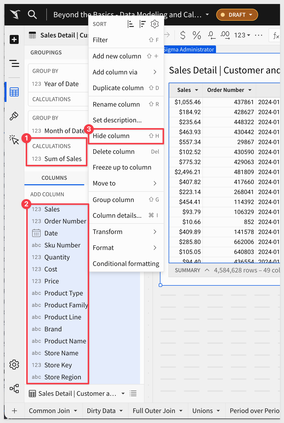
Rename the table to Cumulative Sales.
Our table now shows each year and month, grouped together:
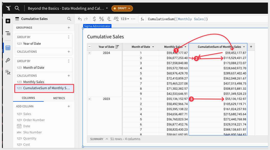
Add another column under Monthly Sales setting the it's formula to:
CumulativeSum([Monthly Sales])
Our table now looks like the screenshot below. Notice how the values in CumulativeSum of Monthly Sales build on the previous cell's value?
For example, the value for 2024-1 just it repeated for CumulativeSum of Monthly Sales.
The value for 2024-2 is added to the the previous CumulativeSum of Monthly Sales value, and so on, until the year changes to 2023, when the pattern restarts:
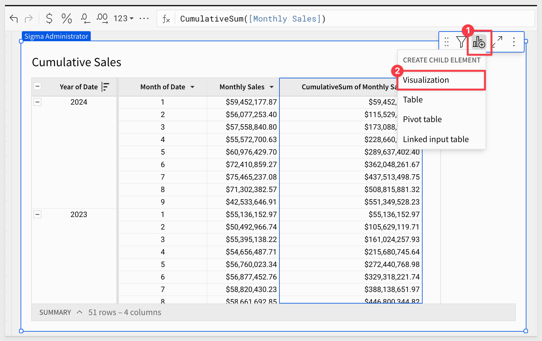
This is pretty cool, but business users would prefer to see this graphically. We can do that with a line chart.
Publish the workbook.
Visualize it
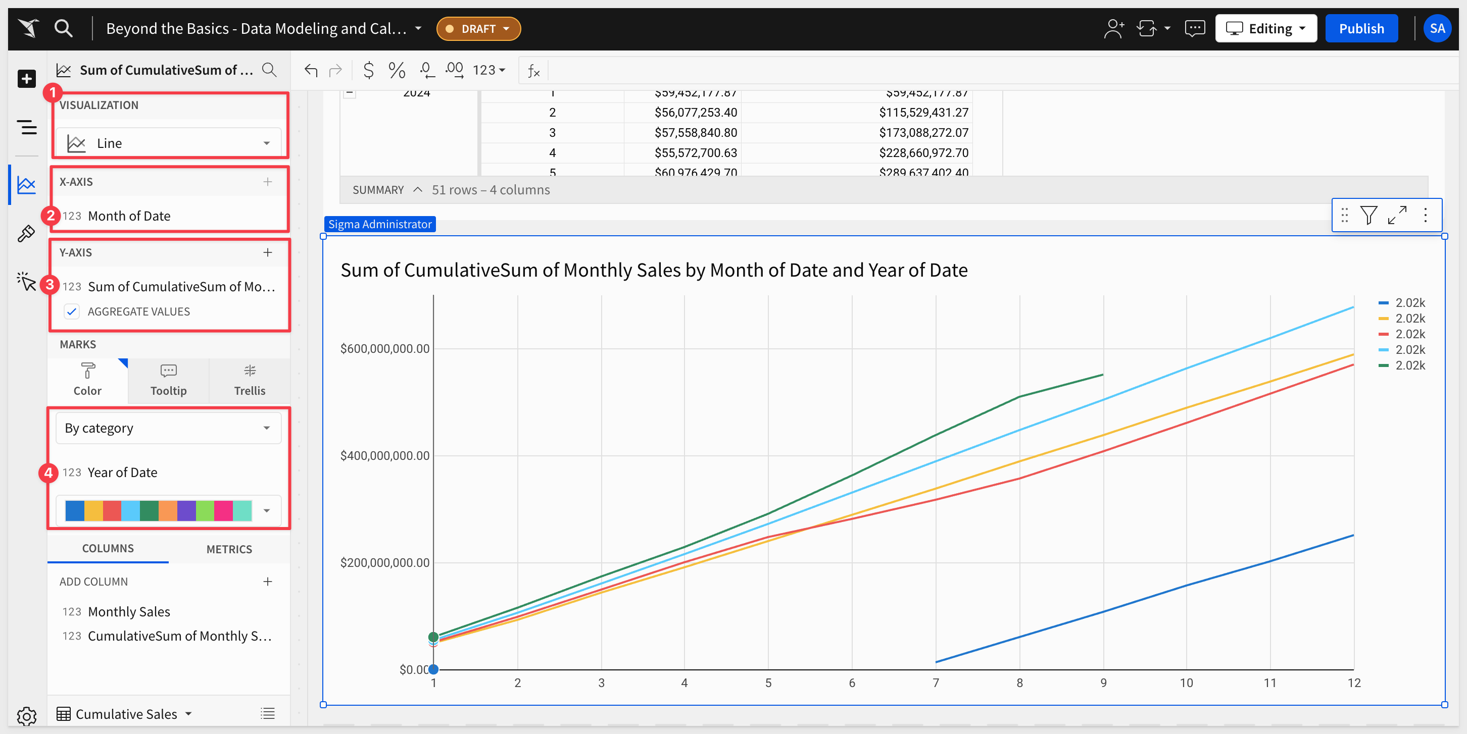
Click to add a Child Visualization from the Cumulative Sales table:
Configure the line chart as shown:
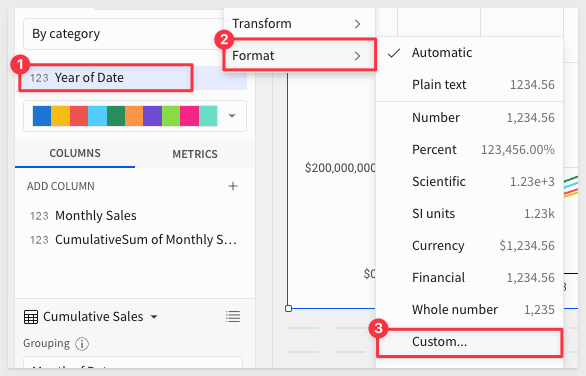
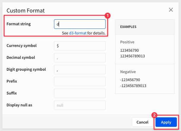
We can clean up the legend formatting of the year:
and
Now, users can easily see how sales are doing year over year and month over month:
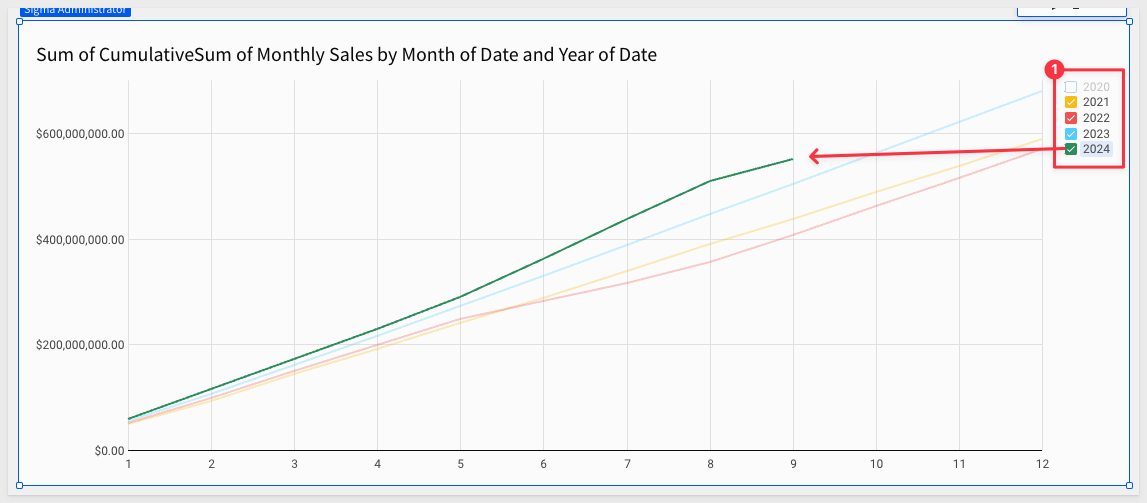
When it goes into a new year, a new data point will be made with a different color, and we never have to touch this chart again, to account for the new year.
Lets take a look at a few areas of using pivot tables that customers contacting Sigma support frequently ask about.
Setup our pivot
Create a new page in our Beyond the Basics - Data Modeling and Calculations workbook, and rename it to Pivot Table.
Add a new PIVOT TABLE element to the page, reusing the Sales Detail | Customer and Store Demographics table on the Common Join page.
Configure the new pivot as shown:
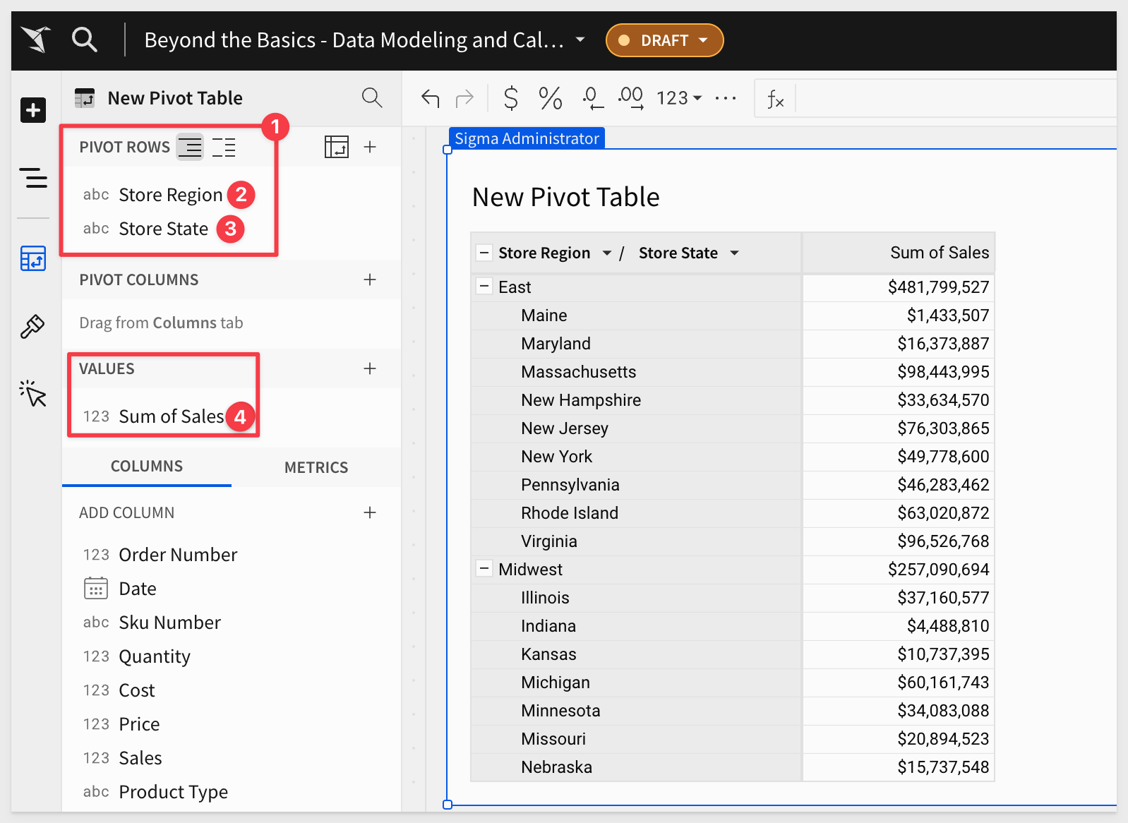
At this point, we have a simple pivot table.
Expose background calculations as columns
Add a another copy of the Sales column, in the VALUES section:
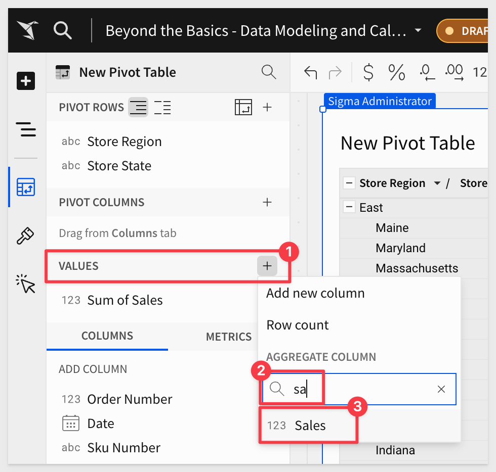
Change the column's formula by typing in [Sales and selecting [Sum of Sales (Row Total)] from the list of available:
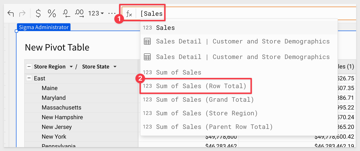
Repeat the process, adding [Sum of Sales (Parent Row Total)] and [Sum of Sales (Grand Total)].
After a little column renaming, our table looks like this:
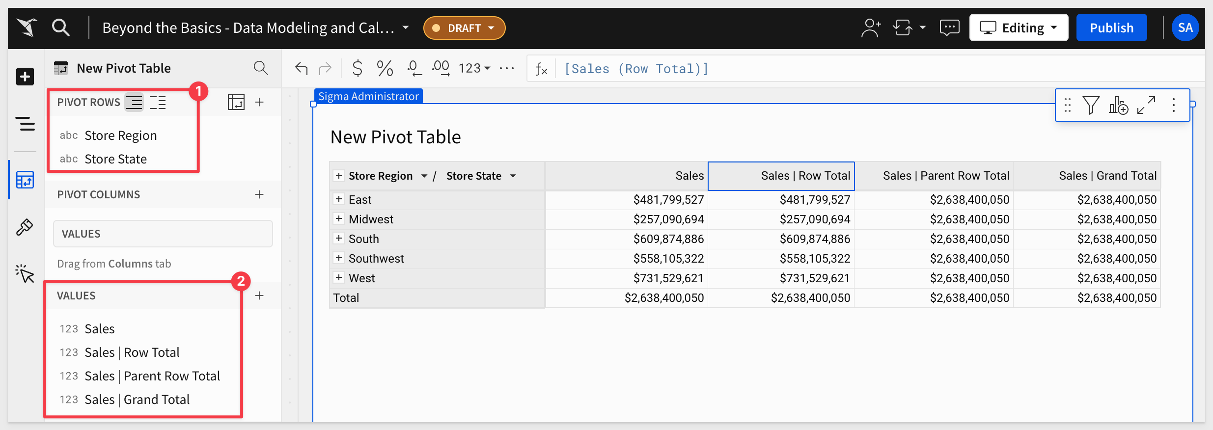
Publish the workbook.
So this is mildly interesting, but how are these automatically generated values useful in practice?
Use background calculations in a pivot
Duplicate the existing pivot table, renaming the new one to Sales with Contribution:
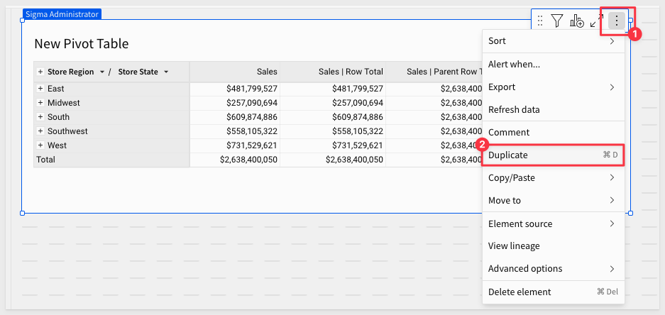
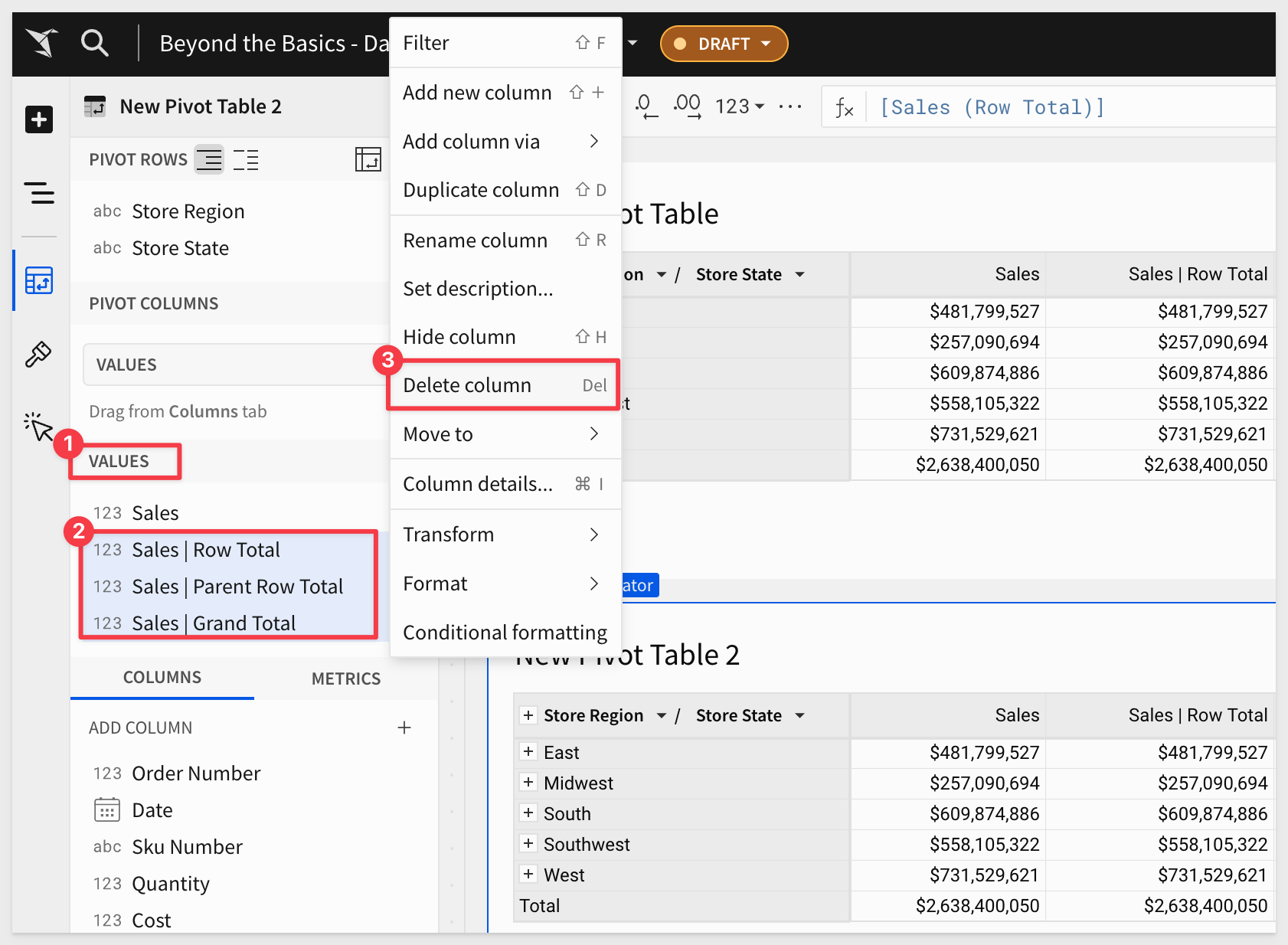
Delete the three extra columns in the VALUES element panel, leaving Sales:
Out pivot currently shows sales at both the Store Region and Store State level.
Lets assume we also want to know what each region and states contribution is to that Total of $2,638,400,050.
We can do that easily by leveraging one of the background calculations that we just reviewed.
Add a new column in the VALUES section of PIVOT COLUMNS and set it's formula to:
Sum([Sales]) / [Sum of Sales (Grand Total)]
Rename the new column Contribution and set its format to Percentage:
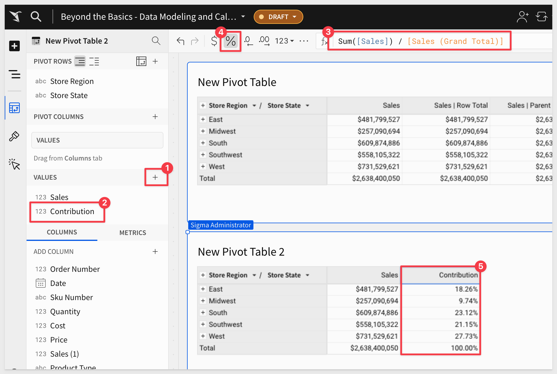
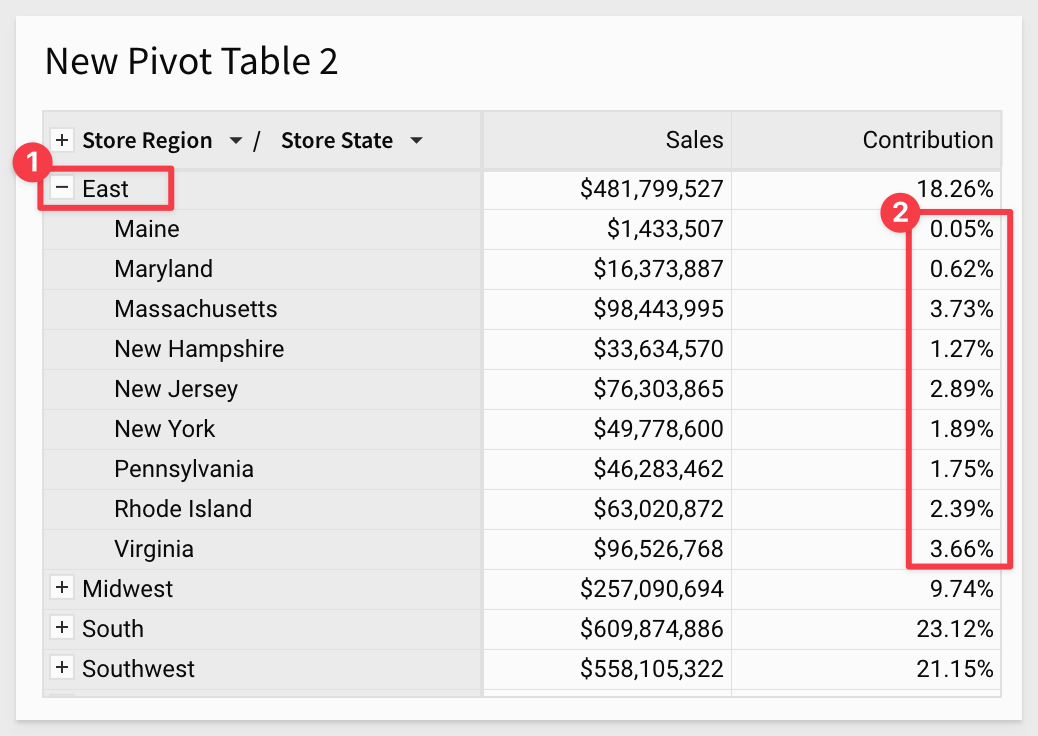
Expanding the East region, we see that the Contribution calculation continues to work for each individual state as well:
Rename the new pivot Contribution to Sales by Region and State and Publish the workbook.
For more information on pivot tables, see Working with pivot tables
There is also a QuickStart, Fundamentals 4: Working with Pivot Tables v2
In this QuickStart, we covered some of the more common questions we receive from Sigma customers.
Additional Resource Links
Blog
Community
Help Center
QuickStarts
Be sure to check out all the latest developments at Sigma's First Friday Feature page!